Munich Personal RePEc Archive
A Generalized Random Regret
Minimization Model
Chorus, Caspar
Delft University of Technology
21 November 2013
A Generalized Random Regret Minimization Model
Caspar G. Chorus
Transport and Logistics Group; Delft University of Technology;
Jaffalaan 5, 2628BX, Delft, The Netherlands
T: +31152788546, F: +31152782719, E: [email protected]
Abstract
This paper presents, discusses and tests a generalized Random Regret Minimization (G-RRM) model. The G-RRM model is created by replacing a fixed constant in the attribute-specific regret functions of the RRM model, by a weight variable. Depending on the value of the regret-weights, the G-RRM model generates predictions that equal those of, respectively, the canonical linear-in-parameters Random Utility Maximization (RUM) model, the conventional Random Regret Minimization (RRM) model, and hybrid RUM-RRM specifications. When the regret-weight variable is written as a binary logit function, the G-RRM model can be estimated on choice data using conventional software packages. As an empirical proof of concept, the G-RRM model is estimated on a stated route choice dataset, and its outcomes are compared with RUM and RRM counterparts.
Keywords: Random Utility Maximization; Random Regret Minimization; Choice model; Unified approach; Generalized Random Regret Minimization.
1. Introduction
Since the introduction of the Random Regret Minimization model (RRM) for discrete choice analysis (Chorus et al., 2008; Chorus, 2010), it has been acknowledged that the model provides a quite different perspective on choice modeling than does discrete choice analysis’ workhorse, the linear-in-parameters Random Utility Maximization (from here on: RUM) model. Particularly, substantial differences have been highlighted in terms of the models’ theoretical properties as well as in terms of their empirical outcomes such as choice probability forecasts and elasticities (e.g., Kaplan & Prato, 2012; Thiene et al., 2012; Boeri et al., 2013; Hensher et al., 2013; Beck et al., 2013; Boeri & Masiero, 2014).
Despite – or perhaps because of – these profound differences, there have also been ongoing attempts to combine the RRM model with the RUM model. Two different approaches can be distinguished: a first approach has been to assume that while some attributes of alternatives are processed in a RRM-fashion, others are processed in a RUM fashion. Resulting so-called hybrid RUM-RRM models have been proposed in Chorus et al. (2013), and applied in, for example, de Bekker-Grob and Chorus (2013) and Leong and Hensher (2014). A second approach has been put forward by Hess et al. (2012) and is based on the assumption that while some decision makers base their decisions on RUM-premises (for all attributes), others use RRM-premises (for all attributes). This approach has been recently applied by Hess & Stathopoulos (2014) and Boeri et al. (2014).
In this paper, an approach to combine the two models is put forward which is fundamentally different from the two approaches mentioned above: I formulate a generalized RRM or form here on G-RRM model, which – in terms of choice probability predictions – nests conventional RUM and RRM models (and hybrid RUM-RRM models) as special cases. By doing so, I show that while the two models – RUM and RRM – obviously may differ substantially in terms of their properties and outcomes, they are more related to one another than is usually thought. The generalization consists of replacing a constant with value ‘1’ in the conventional RRM model, with a so-called regret-weight variable. Depending on the value of the regret-weight variable for a particular attribute, the attribute is processed in a RUM-fashion, an RRM-fashion, or in an intermediate RUM-RRM fashion. By parameterizing these regret-weight variables in binary logit form, the G-RRM model can be easily estimated on standard choice data using conventional software packages. An empirical application is provided, to provide a proof of concept. Note throughout the paper, and without loss of general applicability, the focus is on the logit or MNL form of both the RRM and RUM models.
2. A generalized RRM model (G-RRM)
Since the RRM model has been discussed in detail in a number of previous papers (see for example the papers cited in the introduction), it will be presented here without any accompanying discussion of its model form and properties. The RRM model assumes that decision makers minimize regret when choosing, and that regret of a given alternative is written as follows:
= + = ∑ ∑ ln 1 + exp ∙ − + (1)
denotes the random (or: total) regret associated with a considered alternative
denotes the ‘observed’ regret associated with
denotes the ‘unobserved’ regret associated with , its negative being distributed i.i.d. Extreme Value Type I
denotes the estimable taste parameter associated with attribute
, denote the values associated with attribute for, respectively, the considered alternative and another alternative
As has been widely discussed in recent papers, the main contrast between this RRM model and its linear-in-parameters RUM counterpart (written as = + = ∑ ∙ + , with being distributed i.i.d. Extreme Value Type I) lies in the fact that the RRM model features asymmetric and reference-dependent preferences. More specifically, the RRM model postulates that the extent to which a change in an alternative’s attribute translates into regret depends on how the alternative performs in terms of the attribute, compared to competing alternatives. The poorer the initial relative performance of the alternative in terms of the attribute, the stronger is the impact of a change in attribute value on regret. This reference dependent asymmetry is a direct result of the convexity of the attribute regret function which includes attributes of competing alternatives: ln 1 + exp ∙ − . This function is almost horizontal for
the RRM model such as semi-compensatory behavior and the compromise effect (Chorus & Bierlaire, 2013).
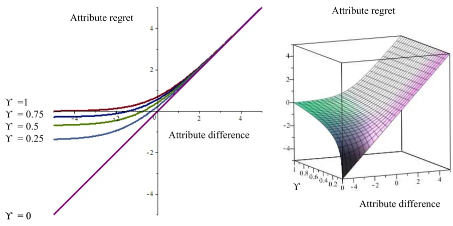
[image:5.595.66.518.347.573.2]The G-RRM model proposed in this paper replaces the ‘1’ in ln 1 + exp ∙ − by a so-called regret-weight variable . By varying from 0 to 1, and plotting the resulting attribute regret function for − ranging from -5 to 5 (keeping fixed at unity), the role of the regret-weight becomes immediately clear; the left hand panel of figure 1 shows the effect on the attribute regret function of a step-wise variation in , and the right hand panel shows the effect of a continuous change in . Both graphs show that when the regret-weight becomes smaller and starts to approach zero, the reference dependent asymmetry in preferences – which is central to the RRM model and its properties – vanishes. When = 0, there is no asymmetry anymore, implying that the impact on regret of a change in an alternative’s attribute is no longer dependent on the alternative’s initial performance in terms of the attribute, relative to its competition.
Figure 1: Impact of variation in regret-weight ( ) on attribute regret (!"=1)
Intuitively, the resulting regret function with symmetric preferences ( = 0) looks like the linear function generated by a linear-in-parameters RUM model, and indeed it can be shown that for = 0, the G-RRM model generates the same choice behavior predictions as does a linear-in-parameter RUM model.
Attribute regret
Attribute difference
ϒ = 0 ϒ = 0 ϒ = 0.25 ϒ = 0.5 ϒ = 0.75 ϒ =1
Attribute difference ϒ
Proposition: given a choice set containing J alternatives, choice probabilities generated by a G-RRM model ( = 0) with parameters of size equal those generated by a linear-in-parameter RUM model with parameters of size # ∙ .
Proof: Note first that when =0, ln + exp ∙ − = ln 0 + exp ∙ − = ∙
− . Now, the regret of alternative i in the G-RRM model (with =0), given parameters , can be written as:
$ % = ∑ ∑ − = ∑ ∑ − $# − 1% ∑
Subtracting from all regrets a constant of size &'()* = ∑ ∑ gives an adapted regret of size +:
+$ % = ∑ ∑ − ∑ ∑ − $# − 1% ∑
= − ∑ − $# − 1% ∑
= −# ∙ ∑
By definition, the utility of i, given parameters of size # ∙ , equals $# ∙ % = ∑ # ∙ = # ∙ ∑ . As a consequence, $# ∙ % = − +$ % = − $ % + &'()*. Noting that the constant drops out when taking the difference, this implies that for any alternative j:
$# ∙ % − $# ∙ % = +$ %− +$ % = $ % − $ %.
Since choice probabilities are fully determined by differences in utility (regret), this proves that choice probabilities of a linear-in-parameter RUM model conditional on parameters of size # ∙ equal those generated by a G-RRM model ( = 0) conditional on parameters of size .
QED
In a practical sense this implies that estimating a G-RRM model (with = 0) gives the same final loglikelihood as a linear-in-parameter RUM model; estimated G-RRM parameters will be J times smaller than their RUM-counterparts. This all in combination establishes that a generalized RRM of G-RRM model which is specified as:
nests – in terms of predicted choice behavior – the conventional RRM model presented in equation (1), and the conventional linear-in-parameter RUM model1. The former model is a special case which is obtained when = = 1 ∀-, and the latter is a special case which is obtained when = = 0 ∀-. Furthermore, hybrid RUM-RRM models of the type Chorus et al. (2013) are also special cases, where ∈ {0,1} ∀-. When ∈]0,1[ ∀-, regret minimization and utility maximization are both co-determinants of choice behavior for the attribute. One more note is in place concerning : since theoretically speaking is bounded between 0 and 1,2 it is pragmatic to parameterize the regret-weight in terms of a binary logit function:
= exp $3 % $1 + exp$3 %%⁄ (3).
Parameter 3 in turn can be treated as a dependent variable, with socio-demographic variables and contextual factors as independent variables, to help explain the determinants of regret minimization versus utility maximization behavior for different attributes. For (large) negative values of 3 , the RUM model is approached for the attribute, and for (large) positive values, the RRM model is approached. When 3 = 0 (or estimated to be insignificantly different from zero), regret minimization and utility maximization are equally important determinants of choice behavior for the attribute.
1
Beyond this equivalence between the G-RRM model with = 0 and the linear-in-parameters RUM model in terms
of (rescaled) parameters and choice probabilities, there is also a very close relation between the two models in terms of economic appraisal metrics. More specifically, it can be easily shown that application, based on +, of the RRM-based marginal rate of substitution measure that was proposed in Chorus (2012a) gives the same result as does its linear-in-parameters RUM- counterpart. Furthermore, application, based on +, of the RRM-LogSum that was proposed in Chorus (2012b) gives the same result (though of course with opposite sign) as does the linear-in-parameters RUM-LogSum.
2
Actually, the G-RRM model can also work with values of greater than 1. This leads to a decrease in sensitivity for situations where a competing alternative outperforms the considered one; in fact, the regret function becomes horizontal very quickly after the Y-axis is crossed for ≫ 1 (as opposed to gradually for = 1). Also for situations where a competing alternative is outperformed by the considered one, the regret function becomes (much) less sensitive to changes in attribute values, especially when the difference in performance is small. Finally, since by
definition the value of the regret function when ∙ − = 0 equals ln(1+ ), the resulting regret function
is shifted upward for values of ∙ − that are either close to (but larger than) zero, equal to, or smaller
3. An empirical proof of concept
This section puts the G-RRM model to the test empirically. Importantly, I do not wish to focus on, or draw any conclusions concerning, the performance of the model relative to conventional RRM and RUM models. Not only can such a judgment only be made after many more empirical tests have been performed, but – more importantly – the G-RUM models is not being put forward here as potentially superior (in terms of empirical performance) to one or both of the RRM or linear-in-parameter RUM models. Rather, the model is presented here as a framework to connect the two model types, and as a means to better understand the relation between them. In that sense, the aimed for contribution of this paper is theoretical, more than empirical. Nonetheless, the empirical application of the unified model is of course important for matters of (face) validity.
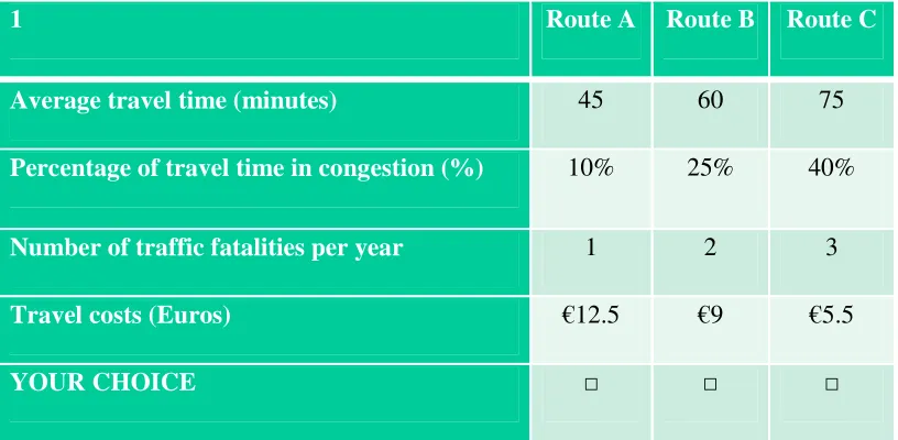
3.1. The data
1 Route A Route B Route C
Average travel time (minutes) 45 60 75
Percentage of travel time in congestion (%) 10% 25% 40%
Number of traffic fatalities per year 1 2 3
Travel costs (Euros) €12.5 €9 €5.5
[image:9.595.95.503.106.306.2]YOUR CHOICE □ □ □
Figure 2: An example route choice-task
3.2. Empirical analysis
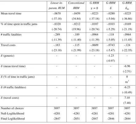
A series of models were estimated using Biogeme (Bierlaire 2003, 2008); estimation results are reported in Table 1: a linear-in-parameters RUM model; a conventional RRM model; a G-RRM model with fixed at zero for all attributes; a G-RRM model with generic value for 3, and a G-RRM model with attribute specific values 3 . Based on the results reported in Table 1, a series of observations can be made.
Table 1: estimation results (robust t-values between brackets) Linear-in-param. RUM Conventional RRM G-RRM = 0 G-RRM 3 G-RRM 3
Mean travel time -.0670
(-37.18) -.0459 (34.84) -.0223 (-37.18) -.0280 (-5.04) -.0225 (-36.86)
% of time spent in traffic jams -.0320
(-20.74) -.0212 (19.96) -.0107 (-20.74) -.0103 (-5.29) -.0169 (-21.19)
# traffic fatalities -.289
(-11.39) -.189 (-11.40) -.0964 (-11.39) -.118 (-5.05) -.0964 (-11.45)
Travel costs -.183
(-23.18) -.115 (-21.99) -.0609 (-23.18) -.0743 (-5.47) -.124 (-22.35)
3 (generic) - - - -1.23
(-0.97)
-
3 (mean travel time) - - - - -6.96
(-2.51)
3 (% of time in traffic jams) - - - - 0
ns3
3 (# traffic fatalities) - - - - -6.23
(-10.49)
3 (travel costs) - - - - 7.10
(7.48)
Number of choices
Null-Loglikelihood Final Loglikelihood 3897 -4281 -2847 3897 -4281 -2851 3897 -4281 -2847 3897 -4281 -2846 3897 -4281 -2844
However, more interestingly than these differences in final loglikelihood is a discussion of parameter estimates. It turns out that three out of four parameters 3 are significantly different from zero. Attributes ‘mean travel time’ and ‘# traffic fatalities’ appear to be processed almost entirely (more precisely, for more than 99%) as a RUM attribute, while attribute ‘travel cost’ is processed almost entirely (for more than 99%) as an RRM attribute. The insignificance of parameter 3 for the attribute ‘% of time in traffic jams’ implies that for this attribute, utility maximization and regret-minimization are equally important co-determinants of choice behavior. In line with expectations, taste parameter values ( s) for ‘utility-attributes’ are very similar to their counterparts in the G-RRM model with =0, while the taste parameter value for the
attribute’ is of similar magnitude as its RRM counterpart. In combination, these findings suggest that the G-RRM model can be estimated on choice data, and that it provides meaningful outcomes that can be unambiguously interpreted in relation to the outcomes of RUM and RRM models.
4. Conclusions
This paper shows how the canonical linear-in-parameters Random Utility Maximization model, and the more recently proposed Random Regret Minimization model, are more closely connected than one might think when inspecting the often substantial differences between these two models. I show how the two models (and hybrid combinations thereof) can – in terms of choice behavior predictions – be conceived as both originating from a generalized RRM or G-RRM model. This G-G-RRM model is created by replacing a constant in the conventional G-RRM model with a regret-weight variable. By parameterizing this regret-weight, the G-RRM model can be estimated empirically on choice data. Although the contribution of this paper is mostly theoretical (i.e. highlighting the connection between the RUM and RRM models), an empirical proof of concept is provided in the form of an empirical estimation of the G-RRM model on a stated route choice dataset. Estimation results are in line with theoretical expectations, and show that the G-RRM model can be used in practice.
A number of directions for further research come to mind: first, it is worthwhile to see how the G-RRM model (and different variants thereof) perform on other datasets. My own experience is that this may vary across datasets in that in a minority of cases convergence issues may arise. This is not entirely unexpected, as empirical identification of the regret-weight parameters, simultaneously with taste parameters, may in some cases by complicated due to the fact that both have an impact on the sensitivity of choice probabilities with respect to variation in the corresponding attribute. To what extent this joint impact can be disentangled into a taste component and a regret-weight component, is likely to depend to some extent on the specifics of the dataset at hand. It may be expected that further parameterization of regret-weights can help in this regard: making them dependent on covariates such as socio-demographic variables and/or contextual variables should help identify parameters.
ad-hoc way of model specification. However, by first estimating the G-RRM model one can easily identify which attribute is more likely to be processed as a utilitarian or regret-based attribute. This information can then be used in a second modeling step which consists of specifying the most likely hybrid RUM-RRM model.
Acknowledgement
Support from The Netherlands Organization for Scientific Research (NWO), in the form of VIDI-grant 016-125-305, is gratefully acknowledged. Discussions with Theo Arentze, Sander van Cranenburgh, Eric Molin and Bert van Wee based on a draft version of this paper, were helpful.
References
Beck, M.J., Chorus, C.G., Rose, J.M., 2013. Vehicle purchasing behaviour of individuals and groups: Regret or reward? Journal of Transport Economics and Policy, 47(3), 475-492
de Bekker-Grob, E.W., Chorus, C.G., 2013. Random regret minimization: A new choice model for health economics. PharmacoEconomics, 31(7), 623-634
Bierlaire M (2003) Biogeme: A free package for the estimation of discrete choice models,
Proceedings of the 3rd Swiss Transportation Research Conference, Ascona, Switzerland.
Bierlaire M (2008) An introduction to BIOGEME Version 1.7, biogeme.epfl.ch
Boeri, M., Longo, A., Grisolia, J.M., Hutchinson, W.G., Kee, F., 2013. The role of regret minimization in lifestyle choices affecting the risk of coronary heart disease. Journal of Health Economics, 32(1), 253-260
Boeri, M., Masiero, L., 2014. Regret minimization and utility maximization in a freight transport context: An application from two stated choice experiments. Transportmetrica (accepted for publication)
Boeri, M., Scarpa. R., Chorus, C.G., 2014. Stated choices and benefit estimates in the context of traffic calming schemes: utility maximization, regret minimization, or both? Transportation Research Part A (conditionally accepted for publication)
Chorus, C.G., Arentze, T.A., Timmermans, H.J.P., 2008. A Random Regret Minimization model of travel choice. Transportation Research Part B, 42(1), 1-18
Chorus, C.G., 2012a. Random Regret Minimization: An overview of model properties and empirical evidence. Transport Reviews, 32(1), 75-92
Chorus, C.G., 2012b. Logsums for utility-maximizers and regret-minimizers, and their relation with desirability and satisfaction. Transportation Research Part A, 46(7), 1003-1012
Chorus, C.G., Bierlaire, M., 2013. An empirical comparison of travel choice models that generate compromise effects. Transportation, 40(3), 549-562
Chorus, C.G., Rose, J.M., Hensher, D.A., 2013a. Regret minimization or utility maximization: It depends on the attribute. Environment and Planning Part B, 40, 154-169
Dekker, T., Chorus, C.G., under review. Insights into value of time for random regret minimization models
Hensher, D.A., Greene, W.H., Chorus, C.G., 2013. Random Regret Minimization or Random Utility Maximization: An exploratory analysis in the context of automobile fuel choice. Journal of Advanced Transportation, 47(7), 667-678
Hess, S., Stathopoulos, A., Daly, A.J., 2012, Allowing for heterogeneous decision rules in discrete choice models: an approach and four case studies, Transportation, 39(3), 565-591.
Hess, S., Stathopoulos, A., 2014. A mixed random utility – random regret model linking the choice of decision rule to latent character traits. Journal of Choice Modelling (conditionally accepted for publication)
Kaplan, S., Prato, C.G., 2012. The application of the random regret minimization model to drivers’ choice of crash avoidance maneuvers. Transportation Research Part F, 15(6), 699-709
Leong, W., Hensher, D.A., in press. Is route choice a matter of regret minimization or relative advantage maximization? Journal of Transport Economics and Policy (conditionally accepted for publication)