Munich Personal RePEc Archive
Factor double autoregressive models with
application to simultaneous causality
testing
Guo, Shaojun and Ling, Shiqing and Zhu, Ke
Academy of Mathematics and Systems Science, Chinese Academy of
Sciences, Hong Kong University of Science and Technology, Academy
of Mathematics and Systems Science, Chinese Academy of Sciences
9 November 2013
Factor double autoregressive models with application to
simultaneous causality testing
BYSHAOJUNGUO
Institute of Applied Mathematics, Chinese Academy of Sciences, Haidian District,
Zhongguancun, Beijing, China 5
SHIQINGLING
Department of Mathematics, Hong Kong University of Science and Technology, Clear Water Bay, Kowloon, Hong Kong
ANDKEZHU
Institute of Applied Mathematics, Chinese Academy of Sciences, Haidian District, Zhongguancun, Beijing, China
ABSTRACT 15
Testing causality-in-mean and causality-in-variance has been largely studied. However, none of the tests can detect causality-in-mean and causality-in-variance simultaneously. In this arti-cle, we introduce a factor double autoregressive (FDAR) model. Based on this model, a score test is proposed to detect causality-in-mean and causality-in-variance simultaneously. Further-more, strong consistency and asymptotic normality of the quasi-maximum likelihood estimator 20
(QMLE) for the FDAR model are established. A small simulation study shows good perfor-mances of the QMLE and the score test in finite samples. A real data example on the causal relationship between Hong Kong stock market and US stock market is given.
Some key words: Asymptotic Normality; Causality-in-mean; Causality-in-variance; Factor DAR model; Instantaneous
causality; Score test; Strong consistency. 25
1. INTRODUCTION
Since the seminal work of Granger (1969), the Granger causality test has been broadly used in finance and economics. Principally, it tells us whether the past information of some specified series can improve the prediction of the current and future values of the other series. The study of causality is of theoretical interest; see, e.g., Geweke (1984a) and Gouri´eroux and Monfort 30
(1997) for earlier works and Nishiyama, Hitomi, Kawasaki, and Jeong (2011) and the references therein for more recent ones. In practice, the causality-in-mean has been widely identified be-tween many macroeconomic variables, e.g., Sims (1972, 1980), Geske and Roll (1983), Ram and Spencer (1983), Stock and Watson (1989), and Lee (1992) to name a few. Recently, the nonlinear causality has received more attention. As a special case of the nonlinear causality, the 35
across different assets or markets; see, e.g., Baillie and Bollerslev (1990), Engle, Ito, and Lin (1990), Hamao, Masulis, and Ng (1990), Ng (2000), and Hong (2001). For more discussions on the explanation of causality-in-variance, we refer to Ross (1989) and Hong (2001).
Testing causality-in-mean and causality-in-variance has been largely but separately studied.
40
For the causality-in-mean, Granger(1969) constructed a F-test based on the regression; Geweke (1982, 1984b) measured the linear dependence including causality-in-mean for the multiple time series; Boudjellade, Dufour, and Roy (1992) gave a testing procedure for the vector ARMA model; and many others. For the causality-in-variance, Cheung and Ng (1996) proposed a resid-ual cross-correlation function test (CCF test); Hong (2001) modified the CCF test by adding the
45
weight function; Hafner and Herwartz (2006) gave a Wald test for the multivariate GARCH model; see also Hiemstra and Jones (1994) and Nishyama et al. (2011) for other nonlinear tests. However, none of the tests aforementioned can detect in-mean and causality-in-variance simultaneously. The empirical studies have demonstrated that these two causality patterns may co-exist; see, e.g., Hamao et al. (1990), Cheung and Ng (1996), and Ng (2000).
Pan-50
telidis and Pittis (2004) showed that without filtering out in-mean, the test for causality-in-variance could suffer severe size distortions in the present of causality-in-mean. Therefore, it urges us to develop a tool to detect them simultaneously.
In this paper, we introduce a factor double autoregressive (hereafter FDAR) model. This causal model not only includes Granger’s linear causality model as a special case, but characterizes the
55
causality-in-variance. An extended FDAR model is also presented to capture the instantaneous causality-in-mean and causality-in-variance altogether. We next propose a score test to detect causality-in-mean and causality-in-variance simultaneously. In presence of both causalities, we propose a quasi-maximum likelihood approach to estimate the parameters in the FDAR model. Under regularity conditions, strong consistency and asymptotic normality of the quasi-maximum
60
likelihood estimator (QMLE) for the FDAR model are obtained. On the basis of this FDAR model, we analyze the causal relationship between Hong Kong stock market and US stock mar-ket. The results find evidence that US stock market affects HK stock market largely in both mean and variance of returns, while the impact of HK stock market to US stock market is relatively weak. This is consistent with our sense, since US market is the largest capital market in the
65
world.
The remainder of the paper is organized as follows. In Section 2, we introduce the FDAR model and give a sufficient and necessary condition for testing in-mean and in-variance. In Section 3, we propose a score test to detect in-mean and causality-in-variance, simultaneously. The asymptotic properties of the QMLE for the FDAR model are
70
studied in Section 4. A simulation study is carried out in Section 5 to examine the performances of the score test and the QMLE in finite samples. A real example is offered in Section 6. All of the proofs are provided in the Appendix.
2. THE CAUSAL MODEL
Suppose that we observe two seriesxt andyt and consider how yt causes xt. Let I1,t and 75
I2,t be σ-fields of{xt} and{yt} available at periodt, respectively. DenoteIt=σ(I1,t,I2,t).
Following Granger (1969),ytis said to causextin mean if
P{E(xt|I1,t−1)≠ E(xt|It−1)}>0. (1)
Next, following Granger, Robins, and Engel (1986),ytis said to causextin variance if
P{E{[xt−E(xt|It−1)]2|I1,t−1}≠ E{[xt−E(xt|It−1)]2|It−1} }>0. (2)
The causality-in-mean, as a special case of linear causality, is often called the first order causality; see Nishyama et al. (2011). The causality-in-variance is a kind of the nonlinear causality defined by Hiemstra and Jones (1994). Both of them are also two special cases of general causalities defined by Granger (1980). It is easy to see that any of (1) and (2) holds if and only if
P{E{[xt−E(xt|I1t−1)]2|I1t−1}̸=E{[xt−E(xt|It−1)]2|It−1} }>0. (3) 85
Thus, testing (1)-(2) altogether is equivalent to testing (3). See also Comte and Lieberman (2000). However, without any other information, (3) can hardly be testable. For instance, it may cause the curse of dimensionality if the conditional expectationE(xt|It−1)is estimated
nonparamet-rically.
To make (3) easily testable, a natural approach is to specify a meaningful causal relationship 90
betweenxtandyt. In this article, we assume that given{(xs, ys), s < t},xt’s are generated from
the following model
xt=φ0+
p ∑
i=1
φixt−i+ q ∑
i=1
ψiyt−i+ηt v u u tα0+
p ∑
i=1
αix2t−i+ q ∑
i=1
βiyt2−i, (4)
where allαi andβi are non-negative constant parameters, {ηt} is a sequence of i.i.d.random
variables with zero mean and unit variance andηtis independent ofIt−1for eacht≥1. We call 95
model (4) as the factor double autoregressive (FDAR) model. When allαi andβi are zeros, it
reduces to the Granger’s linear causal model. When the factorytis absent, it reduces to the DAR
model in Weiss (1986) and Ling (2004, 2007), and furthermore, it reduces to the ARCH model in Engle (1982) if allφi’s are zeros. Throughout the paper, we assume that(xt, yt)are stationary
and ergodic. 100
Since our main goal here is to detect how yt causes xt, we do not specify the generation
mechanism ofyt, whether or not dependent ofxt, only assuming thatytis stationary and ergodic.
Of course, the seriesytcan be modeled in practice. In the end of this section, we give a remark of
how to modelyt. In simulation studies, we choose three generation mechanisms ofyt, showing
that all the procedures proposed in Sections 3 and 4 work well. 105
Based on model (4) and Assumption 1 below, an equivalent but testable condition for (3) is derived.
Assumption1. (i)yt−i̸∈σ(I1,t−1,I2,t−i−1)for anyi≥1; (ii)E|ηt|2 <∞,E|xt|2<∞and
E|yt|2 <∞.
We now give our first proposition, which presents a sufficient and necessary condition for 110
testing (3) under model (4).
PROPOSITION1. Suppose that Assumption1holds. Then, the inequality (3) holds if and only if someψi orβi is not zero. Particularly, (1) holds if and only if some ψi is not zero; and (2) holds if and only if someβiis not zero.
Proof. See Appendix A. 115
Although model (4) captures the causality-in-mean and causality-in-variance simultaneously from yt to xt, it is often meaningful to describe the instantaneous causality-in-mean and
extended FDAR model:
xt=φ0+
p ∑
i=1
φixt−i+ q ∑
i=0
ψiyt−i+ηt v u u tα0+
p ∑
i=1
αix2t−i+ q ∑
i=0
βiy2t−i, (5) 120
where all αi, βi, and {ηt} are defined as in model (4) except that ηt is independent of
σ(I1,t−1,I2,t). Clearly, the extended FDAR model reduces to FDAR model whenψ0=β0 = 0.
As in Hong (2001), we say that there is an instantaneous causality-in-mean betweenxtandytif
P{E(xt|It−1)̸=E(xt|I1,t−1,I2,t)}>0 (6)
and an instantaneous causality-in-variance betweenxtandytif 125
P{E{[xt−E(xt|I1,t−1,I2,t)]2|It−1}̸=E{[xt−E(xt|I1,t−1,I2,t)]2|I1,t−1,I2,t }}
>0. (7)
Analogous to Proposition 2.1, our second proposition below gives a sufficient and necessary condition for testing (6) and (7) under model (5) and Assumption 2.
Assumption2. (i)yt̸∈ It−1; (ii)E|ηt|2 <∞,E|xt|2<∞andE|yt|2 <∞.
PROPOSITION2. Suppose that Assumption 2 holds. Then, relation (6) holds if and only if 130
ψ0 ̸= 0; and relation (7) holds if and only ifβ0 ̸= 0.
Proof. The proof is directly from Assumption 2 and hence omitted.
Till now, we have not restricted the specification ofyt. Although not being necessary, it is also
worthwhile to modelytby an extended FDAR model in practice, especially whenytexhibits the
conditional heteroskedasticity. That is, we consider another extended FDAR model foryt: 135
yt=π0+
r ∑
i=0
πixt−i+ s ∑
i=1
ωiyt−i+ζt v u u tτ0+
r ∑
i=0
τix2t−i+ s ∑
i=1
νiyt2−i. (8)
Likewise, model (8) shares the same property as model (5). In what follows, we call models (5) and (8) as the bivariate extended FDAR model. Based on this bivariate extended FDAR model, Assumptions 1-2 hold ifηtandζtare independent. Intuitively, ifηtandζtare dependent, there
may exist either a common factor zt affecting both xt andyt, or some other nonlinear causal 140
relation besides the causality-in-variance between xt andyt. In this case, we suggest to use a
multivariate extended FDAR model to deal with the problem of common factors. If ηtand ζt
remain dependent after filtering out the impact of common factors, a further nonlinear test in Hiemstra and Jones (1994) can be implemented to detect whether there are some other nonlinear causal relations besides the causality-in-variance.
145
3. SIMULTANEOUS CAUSALITY TEST
In this section, we propose a score test to simultaneously detect the causality-in-mean and causality-in-variance fromyttoxtunder model (4). We first assume that bothpandqare known.
In the end of this section, the case thatpandqare unknown is discussed. Letθ= (φ′, ψ′, α′, β′)′ be the unknown parameters of model (4), where φ= (φ0,· · · , φp)′, α= (α0,· · · , αp)′, ψ= 150
hypotheses:
H0 :ψ≡β ≡0. (9)
Given the observations {(xt, yt)}nt=1, we denoteXt= (1, xt−1,· · ·, xt−p)′,Xt∗ = (1, x2t−1,
· · ·, x2t−p)′, Yt= (yt
−1,· · · , yt−q)′ and Yt∗ = (yt2−1,· · · , yt2−q)′. By assuming that ηt follows 155
standard normal distribution, the quasi-log-likelihood function (ignoring a constant) of model (4) is:
Ln(θ) =−
1
n
n ∑
t=m
lt(θ) and lt(θ) = log √
ht(θ) +
ε2t(θ) 2ht(θ)
, (10)
wherem= 1 +max(p, q),εt(θ) =xt−φ′Xt−ψ′Ytandht(θ) =α′Xt∗+β′Yt∗. Here,ht(θ)
is the conditional variance ofxt, givenIt−1. 160
Under H0, model (4) becomes a DAR(p) model with parameters (φ′, α′)′. Denote Θ1=:
Θφ×Θα be the parameter space of this DAR(p) model. Let θ¯10=: ( ¯φ′0,α¯′0)′ be the true
value of (φ′, α′)′ ∈Θ1. As in Ling (2007), the quasi-maximum likelihood estimator (QMLE)
ˆ
θ1n=: ( ˆφ′n,αˆ′n)′ forθ¯10is obtained by maximizingLn(θ)with respect to(φ′, α′)′∈Θ1 under
the constraint that(ψ′, β′)≡0. Moreover, letθˆn= ( ˆφ′
n,01×q,αˆn′,01×q)′ and 165
Tn(θ) = (
∂Ln(θ)
∂ψ′ ,
∂Ln(θ)
∂β′
)′
(11)
be the score function forψandβ. To construct the score statistics, we desire to prove thatTn(ˆθn)
is asymptotically normal with mean zero underH0 and regularity conditions. To accomplish it,
we need the following two assumptions.
Assumption3. θ¯10is an interior point inΘ1, andΘ1is compact withαLi ≤αi ≤αUi for alli, 170
whereαL
i andαUi are some positive constants.
Assumption4. E|ηt|4<∞,E|xt|ι <∞for someι >0, andE|yt|4 <∞.
To be convenient, we make some notations before the theorem:
J =
1 −
Eη3 t √
2
−Eη
3 t √
2
Eη4 t−1
2
and At(¯θ10) =diag
{
Γ1Xt−Yt √
ht(¯θ0)
,Y√t∗−Γ2Xt∗
2ht(¯θ0)
}
, (12)
whereθ¯0= ( ¯φ′0,01×q,α¯′0,01×q)′,
Γ1=E
(
YtXt′
ht(¯θ0)
) [
E
(
XtXt′
ht(¯θ0)
)]−1
and Γ2 =E
(
Y∗
t X∗
′
t
h2
t(¯θ0)
) [
E
(
X∗
tX∗
′
t
h2
t(¯θ0)
)]−1
.
Then, we can give our first main result as follows: 175
THEOREM1. Suppose that Assumptions 1(i) and 3-4 hold and J is positive definite. Then, underH0, asn→ ∞,
√
nTn(ˆθn)→dN(0,Ξ),
where →d denotes the convergence in distribution, Ξ =E[At(¯θ10)JA′t(¯θ10)], and J and
At(¯θ10)are defined in (12). 180
It is important to point out that Γ1 and Γ2 are both well defined, since the matrixes
E[XtXt′/ht(¯θ0)]andE
[
X∗
tX∗
′
t /h2t(¯θ0)
]
are positive definite by Lemma B.5 in Ling (2007).
Also, it is readily shown thatJ >0if and only if P(ηt2−cηt−1 = 0)<1for anyc∈R. A
simple condition for this is thatηt has a positive density on some interval. In particular, when 185
ηt∼N(0,1),J becomes the identity matrix.
In practice, given the observations{(xt, yt)}nt=1, the matrixΞcan be consistently estimated
by its sample meanΞbn. UnderH0, if the conditions in Theorem 1 hold, it is not hard to show
thatΞbn= Ξ +op(1). Therefore, we construct a score test statistic
Sn=nTn′(ˆθn)Ξb−n1Tn(ˆθn)
to test (9). The following corollary gives its asymptotic distribution, as expected.
COROLLARY1. Suppose that the conditions in Theorem1hold. Then, underH0, asn→ ∞,
Sn→dχ22q,
whereχ2kis a chi-square distribution with degree of freedomk.
Proof. The proof is directly from Theorem 1, and hence it is omitted.
Remark1. Based on model (5), a score testS⋄
nwhich is similar toSn, can be used to detect
the hypothesis
H⋄
0 :θ⋄2 ≡0,
whereθ⋄
2 = (ψ′, β′, ψ0, β0)′. If Assumption 2(i) and the conditions in Theorem 1 hold, by using
190
the same method as in Corollary 1, we can easily show that underH⋄
0,Sn⋄ converges toχ22(1+q)
asn→ ∞.
Indeed, the test statisticSn always depends on the orders p andq. Without confusion, we
shorten the notation Sn(p, q) toSn for brevity. In practice, bothp and q are often unknown,
and should be determined before usingSn. This can be done by Akaike’s information criterion 195
(AIC). In this case, we propose our testing procedure as follows:
1. Determine the values ofpandqby AIC under FDAR model (4).
2. Calculate the test statistic Sn and compare it to the upper-tailed critical value ofχ22q at an
appropriate level.
3. IfSnis larger than the critical value, then the null hypothesisH0is rejected. Otherwise,H0
200
is not rejected.
Clearly, the above procedure is also applicable to detectH⋄
0 via replacingSnandχ22qby Sn⋄
andχ2
2(1+q), respectively. In order to accomplish Step 1 aforementioned, it is necessary for us
to consider the estimation for the FDAR model. The full study on this topic is given in the next section.
205
4. THE QMLE
In this section, we study the QMLE for model (4). DenoteΘ =: Θφ×Θψ×Θα×Θβ be the
parameter space of model (4), whereΘφ⊂R1+p, Θψ ⊂Rq, Θα ⊂R+1+p andΘβ ⊂Rq+ with
minimizer ofLn(θ)inΘ, i.e., 210
˜
θn= arg max
θ∈Θ Ln(θ). (13)
whereLn(θ)is defined in (10). We callθ˜nbe the QMLE ofθ0. To derive the asymptotic property
ofθ˜n, we make the following assumptions:
Assumption5. The true valueθ0 is an interior point inΘ, andΘis compact withαLi ≤αi ≤
αU
i andβjL≤βj ≤βjU for alliandj, whereαLi ,αUi ,βjLandβUj are some positive constants. 215
Assumption6. E|xt|ι <∞andE|yt|ι<∞for someι >0.
Assumptions 5-6 are analogous to Assumptions 3-4 except that only the fractional moment of yt is required. This is because the conditional variance ht(θ) itself as one sort of weight can
control the log-likelihood function (10). When yt is absent and p= 1 (i.e., DAR(1) model),
Borkovec and Kl¨uppelberg (2001) showed that the conditionE(ln|φ+ηt√α|)<0is sufficient 220
for the stationarity ofxt. Note that this condition doesn’t rule out the case that|φ| ≥1. Hence, it
implies that the stationary region of DAR(1) model is larger than that of AR(1) model; see Ling (2004, 2007) for more discussions on it.
We now are ready to give our second main result as follows:
THEOREM2. Suppose that Assumptions1(i) and5-6hold,Eη4t <∞andJ is positive defi- 225 nite. Then, asn→ ∞,
(i) ˜θn→θ0 a.s.;
(ii)√n(˜θn−θ0)→dN(0,Ω−01Σ0Ω−01),
whereΩ0 =E[Bt(θ0)Bt′(θ0)],Σ0 =E[Bt(θ0)JBt′(θ0)], and
Bt(θ) =
( 1
√
ht(θ)
∂εt(θ)
∂θ′ ,
1
√
2ht(θ)
∂ht(θ)
∂θ′
)′ .
Proof. See Appendix B.
Remark2. Similar to (13), we can define the QMLE θ⋄
n of θ0⋄ for model (5), where θ⋄0 =
(θ′
0, ψ00, β00)′is the true value of model (5). If Assumption 2(i) and the conditions in Theorem 230
2 hold, by using the similar method as for Theorem 2, the strong consistency and asymptotic normality ofθ⋄
ncan be obtained as well.
By a direct calculation, we can see that
∂εt(θ)
∂θ = (−Kt′,01×(p+q))′and
∂ht(θ)
∂θ = (01×(1+p+q), K∗
′
t )′.
whereKt= (Xt′, Yt′)′andKt∗ = (X∗
′
t , Y∗
′
t )′. Thus we can show thatΩ0 >0andΣ0 >0ifJ > 235
0and Assumption 1 holds. Whenytis absent, the asymptotic variance in Theorem 2 is the same
as the one for the DAR(p) models in Ling (2007). Furthermore, ifEηt3= 0, thenΩ−1 0 Σ0Ω−01
reduces to a block diagonal matrix
diag
{[
E
(
1
ht(θ0)
KtKt′ )]−1
, κ·
[
E
(
1 2h2
t(θ0)
K∗
tK∗
′
t
)]−1}
,
withκ= (Eη4
In the end, we proceed to discuss the diagnostic checking of model (4). Denote ηˆt be the
residual of model (4). A portmanteau testQ2(M)defined in the same way as the Li-Mak test can be used to test the independence of{ηt}. If{ηt}is independent, by a similar method as in Li and Mak (1994), we can show thatQ2(M)→dχ2M asn→ ∞. Therefore, model (4) is not adequate
ifQ2(M)is larger than the upper-tailed critical value ofχ2
M at an appropriate level. Moreover, if 245
we further consider a bivariate extended FDAR model, the test statisticC(M) =:n∑Mi= −Mrˆ2i
defined in the same way as the CCF test can be used to detect the independence of {ηt}and {ζt}, whererˆi is the sample cross-correlation of the squared residuals{ηˆ2t}and{ζˆt2}at lagi. If {ηt}and{ζt}are independent, by a similar method as in Cheung and Ng (1996), it is not hard to show thatC(M)→dχ22M+1 asn→ ∞. Hence, we reject the hypothesis that{ηt}and{ζt}are 250
independent, if C(M)is larger than the upper-tailed critical value ofχ2
2M+1 at an appropriate
level.
5. SIMULATION
In this section, we first give a simulation study to assess the performance ofθ˜nin finite
sam-ples. The model used to generate data samples is
255
xt=φ0+φ1xt−1+ψ1yt−1+ηt √
α0+α1x2t−1+β1y2t−1. (14)
whereηtfollows the standard normal distribution. The factor sample{yt}nt=1are generated from
three different models:
(a)yt= 0.5yt−1+ζt (AR(1) model);
(b)yt=ζt √
0.1 + 0.5y2
t−1 (ARCH(1) model);
(c)yt= 0.5yt−1+ 0.5xt−1+ζt √
0.1 + 0.2y2
t−1+ 0.3x2t−1 (FDAR model),
where ζt follows the standard normal distribution and is independent of ηt. We
take the sample size n= 1000 and use 1000 replications. The true parameters are
260
θ0 = (0.0,0.5,0.5,1.0,0.5,0.5), (0.0,0.0,−0.3,1.0,0.5,0.5),(0.0,0.6,0.0,1.0,0.6,0.3), and
(0.0,−0.2,0.7,1.0,0.3,0.6), respectively. Based on models (a)-(c), Tables 1-3 list the sample biases, the sample standard deviations (SD) and the average estimated asymptotic standard devi-ations (AD) ofθ˜n, respectively. Each estimated asymptotic standard deviation is obtained from
Theorem 2 withΩ0 andΣ0being estimated by their sample averages. From Tables 1-3, we can
265
see thatθ˜nhas very small bias and its SD and AD are very close to each other. Interestingly, the
way in which{yt}is generated does not affect the performance ofθ˜n, hence it gives us enough
freedom to choose factor in practice.
Next, we assess the performance of our score test (Sn) in finite samples. The model used to
generate data samples is
270
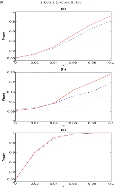
xt= 0.5xt−1+ψ1yt−1+ηt √
1.0 + 0.5x2
t−1+β1yt2−1, (15)
where (ψ1, β1) =κ(1.0,1.0) with κ={0.0,0.02,0.04,· · ·,0.1}, and the factor samples
{yt}nt=1are generated from models (a)-(c). Here,{ηt}nt=1and{ζt}nt=1are random samples
gener-ated from a bivariate normal distribution with mean zero, variance one, and covarianceρ. Again, we set the sample size n= 1000 and use 1000 replications, and choose the significance level
275
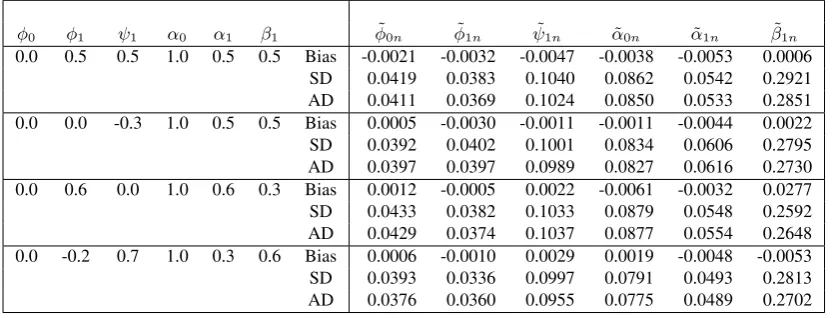
Table 1.Estimators for model (14) when{yt}is generated from model (a)
φ0 φ1 ψ1 α0 α1 β1 φ˜0n φ˜1n ψ˜1n α˜0n α˜1n β˜1n 0.0 0.5 0.5 1.0 0.5 0.5 Bias -0.0012 -0.0027 -0.0009 0.0091 -0.0063 -0.0026
SD 0.0484 0.0351 0.0549 0.1144 0.0505 0.1023 AD 0.0487 0.0356 0.0527 0.1119 0.0489 0.0984 0.0 0.0 -0.3 1.0 0.5 0.5 Bias -0.0019 -0.0017 -0.0010 0.0028 -0.0049 0.0012 SD 0.0466 0.0398 0.0511 0.1072 0.0579 0.0999 AD 0.0462 0.0390 0.0501 0.1059 0.0585 0.0926 0.0 0.6 0.0 1.0 0.6 0.3 Bias -0.0017 -0.0044 -0.0013 -0.0008 -0.0038 -0.0020 SD 0.0461 0.0375 0.0501 0.1069 0.0541 0.0783 AD 0.0476 0.0373 0.0483 0.1077 0.0547 0.0786 0.0 -0.2 0.7 1.0 0.3 0.6 Bias 0.0013 -0.0008 0.0001 -0.0029 -0.0029 -0.0016 SD 0.0449 0.0341 0.0504 0.1033 0.0437 0.0938 AD 0.0446 0.0342 0.0504 0.1007 0.0427 0.0959
Table 2.Estimators for model (14) when{yt}is generated from model (b)
φ0 φ1 ψ1 α0 α1 β1 φ˜0n φ˜1n ψ˜1n α˜0n α˜1n β˜1n 0.0 0.5 0.5 1.0 0.5 0.5 Bias -0.0021 -0.0032 -0.0047 -0.0038 -0.0053 0.0006
SD 0.0419 0.0383 0.1040 0.0862 0.0542 0.2921 AD 0.0411 0.0369 0.1024 0.0850 0.0533 0.2851 0.0 0.0 -0.3 1.0 0.5 0.5 Bias 0.0005 -0.0030 -0.0011 -0.0011 -0.0044 0.0022 SD 0.0392 0.0402 0.1001 0.0834 0.0606 0.2795 AD 0.0397 0.0397 0.0989 0.0827 0.0616 0.2730 0.0 0.6 0.0 1.0 0.6 0.3 Bias 0.0012 -0.0005 0.0022 -0.0061 -0.0032 0.0277 SD 0.0433 0.0382 0.1033 0.0879 0.0548 0.2592 AD 0.0429 0.0374 0.1037 0.0877 0.0554 0.2648 0.0 -0.2 0.7 1.0 0.3 0.6 Bias 0.0006 -0.0010 0.0029 0.0019 -0.0048 -0.0053 SD 0.0393 0.0336 0.0997 0.0791 0.0493 0.2813 AD 0.0376 0.0360 0.0955 0.0775 0.0489 0.2702
that the sizes ofSnare close to their nominal ones. Although the power becomes weaker as the
value ofρincreases,Snperforms well no matter how the factor samples are generated. Overall,
the numerical study shows that bothθ˜nandSnhave good performances in finite samples. 280
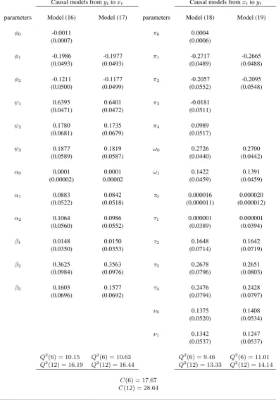
6. AN EXAMPLE
In this section, we study the causal relationship between Hong Kong (HK) stock market and US stock market. We choose the Hang Seng index (HSI) and SP500 Composite index (SPCI) as the proxies for the HK stock market and the US stock market, respectively. The data sets used are the daily closing HSI data and SPCI data from Jun 16, 2008 to Jun 10, 2010, and each of 285
them has in total 501 observations; see Fig 2 (a). Furthermore, we denote the log-return of HSI and SPCI byxtandyt, respectively, and plot them in Fig 2 (b).
We first consider the causal relation fromyttoxt. Unless stated otherwise, we set the
signif-icance levelα= 0.05. According to AIC, we choosep= 2andq = 3in model (4). Then, we obtainSn= 73.6, which is greater than12.59(the 95% upper percentile ofχ26). So there exists 290
[image:10.595.98.516.310.469.2]0 0.02 0.04 0.06 0.08 0.1 0
0.05 0.2 0.4 0.6 0.8 1
κ
Power
(a)
0 0.02 0.04 0.06 0.08 0.1
0 0.05 0.1 0.15 0.2 0.25
κ
Power
(b)
0 0.02 0.04 0.06 0.08 0.1
0 0.05 0.2 0.4 0.6 0.8 1
κ
Power
(c)
Fig. 1. (a) power curves forρ= 0(solid line),ρ= 0.4(dashed line), andρ= 0.8(dotted line), based on model (a);(b) power curves forρ= 0(solid line),ρ= 0.4(dashed line), andρ= 0.8(dotted line), based on model (b);(c) power
[image:11.595.80.470.74.708.2]Table 3.Estimators for model (14) when{yt}is generated from model (c)
φ0 φ1 ψ1 α0 α1 β1 φ˜0n φ˜1n ψ˜1n α˜0n α˜1n β˜1n 0.0 0.5 0.5 1.0 0.5 0.5 Bias 0.0002 -0.0018 -0.0005 -0.0032 -0.0030 -0.0007
SD 0.0714 0.0354 0.0398 0.1406 0.0469 0.0520 AD 0.0697 0.0354 0.0399 0.1362 0.0445 0.0514 0.0 0.0 -0.3 1.0 0.5 0.5 Bias -0.0023 -0.0013 0.0012 -0.0028 -0.0011 -0.0032 SD 0.0498 0.0384 0.0462 0.0989 0.0601 0.0699 AD 0.0483 0.0389 0.0456 0.0987 0.0581 0.0694 0.0 0.6 0.0 1.0 0.6 0.3 Bias 0.0004 -0.0028 0.0007 -0.0048 -0.0041 -0.0013 SD 0.0540 0.0383 0.0370 0.1021 0.0560 0.0426 AD 0.0533 0.0381 0.0373 0.1060 0.0559 0.0426 0.0 -0.2 0.7 1.0 0.3 0.6 Bias 0.0017 -0.0012 -0.0035 -0.0032 -0.0016 -0.0037 SD 0.0516 0.0312 0.0422 0.1026 0.0396 0.0648 AD 0.0514 0.0327 0.0424 0.1018 0.0379 0.0634
1 50 100 150 200 250 300 350 400 450 500 5000
10000 15000 20000 25000
Time (a)
1 50 100 150 200 250 300 350 400 450 500 −0.2
−0.15 −0.1 −0.05 0 0.05 0.1 0.15
Time (b)
the following FDAR model
xt=φ0+ 2
∑
i=1
φixt−i+
3
∑
i=1
ψiyt−i+ηt v u u
tα0+∑2 i=1
αix2t−i+
3
∑
i=1
βiy2t−i, (16)
to fit the data set{xt}. All parameters are estimated through the QMLE method and these results
are reported in Table 4 with the standard errors in parentheses. Based on the residuals {ηˆt}, 295
the Li-Mak tests Q2(6)and Q2(12) reported in Table 4 indicate that model (16) is adequate.
However, the parameters φ0 in model (16) is not significantly different from zero. Hence, by
using the QMLE method, we re-fit the data set{xt}as
xt=
2
∑
i=1
φixt−i+
3
∑
i=1
ψiyt−i+ηt v u u
tα0+∑2 i=1
αix2t−i+
3
∑
i=1
βiyt2−i, (17)
where all results for model (17) are reported in Table 4, and indicate that model (17) is adequate.
300
From this model, we observe that US market affects HK market in both the mean and variance of return. Specifically, the influence for the mean of return lasts for three days, and it becomes weak as time goes by; while the influence for the variance of return has one-day delay sinceβ1
closes to zero, and then starts to mitigate two days later.
Next, we consider the causal relation fromxttoyt. Since HK stock market is one day earlier 305
than US stock market in calendar, we use S⋄
ninstead ofSnin this case. According to AIC, we
choose p= 4 andq= 1 in model (8). Then, we obtain S⋄
n= 127.8, which is greater than9.5
(the 95% upper percentile ofχ2
4). Similar to model (16), we obtain the following fitted model for
the data set{yt}:
yt=π0+ 4
∑
i=1
πiyt−i+
1
∑
i=0
ωixt−i+ζt v u u
tτ0+∑4 i=1
τiy2t−i+
1
∑
i=0
νix2t−i, (18) 310
where all results for model (18) are reported in Table 4, and indicate that model (18) is adequate. Furthermore, we find that the parameters π0, π3, and π4 in model (18) are not significantly
different from zero. Thus, similar to model (17), we re-fit the data set{yt}using the model
yt=
2
∑
i=1
πiyt−i+
1
∑
i=0
ωixt−i+ζt v u u
tτ0+∑4 i=1
τiyt2−i+
1
∑
i=0
νix2t−i. (19)
Again, all results for this adequate model are reported in Table 4. Since the parametersω0,ω1,ν0,
315
andν1 in model (19) are significantly different from zero, we claim that HK market causes US
market in both the mean and variance. However, compared with model (17), the impact period from HK market to US market only lasts for two days, and is shorter than the one from US market to HK market. This is consistent with the fact that the US market is the largest capital market in the world. Moreover, based on the residuals from models (17) and (19), the CCF testsC(6)and
320
Table 4.Results for models (16)-(19)
Causal models fromyttoxt Causal models fromxttoyt
parameters Model (16) Model (17) parameters Model (18) Model (19)
φ0 -0.0011 π0 0.0004
(0.0007) (0.0006)
φ1 -0.1986 -0.1977 π1 -0.2717 -0.2665
(0.0493) (0.0493) (0.0489) (0.0488)
φ2 -0.1211 -0.1177 π2 -0.2057 -0.2095
(0.0500) (0.0499) (0.0552) (0.0548)
ψ1 0.6395 0.6401 π3 -0.0181
(0.0471) (0.0472) (0.0511)
ψ2 0.1780 0.1735 π4 0.0989
(0.0681) (0.0679) (0.0517)
ψ3 0.1877 0.1819 ω0 0.2726 0.2700
(0.0589) (0.0587) (0.0440) (0.0442)
α0 0.0001 0.0001 ω1 0.1422 0.1391
(0.00002) 0.00002 (0.0459) (0.0459)
α1 0.0883 0.0842 τ0 0.000016 0.000020
(0.0522) (0.0518) (0.000011) (0.000012)
α2 0.1064 0.0986 τ1 0.000001 0.000001
(0.0560) (0.0552) (0.0389) (0.0394)
β1 0.0148 0.0150 τ2 0.1648 0.1642
(0.0350) (0.0353) (0.0714) (0.0719)
β2 0.3625 0.3563 τ3 0.2678 0.2651
(0.0984) (0.0976) (0.0796) (0.0803)
β3 0.1603 0.1577 τ4 0.2476 0.2428
(0.0696) (0.0692) (0.0794) (0.0797)
ν0 0.1375 0.1408
(0.0520) (0.0534)
ν1 0.1342 0.1247
(0.0537) (0.0537)
Q2(6) = 10.15 Q2(6) = 10.63 Q2(6) = 9.46 Q2(6) = 11.01
Q2
(12) = 16.19 Q2
(12) = 16.44 Q2
(12) = 13.33 Q2
(12) = 14.14
C(6) = 17.67
ACKNOWLEDGEMENT
The authors gratefully acknowledge the constructive suggestions and comments from the
Ed-325
itor, the Associate Editor and three referees that greatly improve this article. The research of S. Guo was supported by the Chinese NSF grants(Y2110515K1) and Key Lab of Random Com-plex Structures and Data Science of Chinese Academy of Sciences. The research of S. Ling was supported by Hong Kong grants(641912 and 603413, HKUST). The research of K. Zhu was supported by the Chinese NSF grants(11201459) and the National Center for Mathematics and
330
Interdisciplinary Sciences of Chinese Academy of Sciences.
A. PROOF OFPROPOSITION1 PROOF OFPROPOSITION1. For brevity, we only prove that
the inequality(3)fails if and only if allψiandβiare zeros. (A1)
It suffices to show the necessity of (A1). Suppose that relation (3) does not hold. By Assumption 1 and a
335
direct calculation, it follows that
E
( q
∑
i=1
ψiyt−i
)2
I1t−1
−
[
E
( q
∑
i=1
ψiyt−i I1t−1
)]2
+E
( q
∑
i=1
βiyt2−i I1t−1
)
=
q ∑
i=1
βiyt2−i (A2)
a.s. Then, ifβ1̸= 0, we haveyt−1∈σ(I1,t−1,I2,t−2), and this is a contradiction with Assumption 1(i). Hence,β1= 0. Similarly,β2=· · ·=βq= 0. Next, when allβiare zeros, by (A2) and H¨older’s inequal-340
ity, we know that ∑qi=1ψiyt−i ≡constant a.s. Then, if ψ1̸= 0, we haveyt−1∈ I2,t−2, and this is against Assumption 1(i). Hence,ψ1= 0. Similarly,ψ2=· · ·=ψq = 0. This completes the proof.
B. PROOFS OFTHEOREMS1AND2
To facilitate presentation in the proof of Theorem 1, we denoteε˜t(φ) =xt−φ′Xtand˜ht(α) =α′Xt∗
and let
˜
Ln(θ1) =− 1
n
n ∑
t=m
˜
lt(θ1) with ˜lt(θ1) = log
√
˜
ht(α) +
˜
ε2
t(φ)
2˜ht(α)
,
whereθ1= (φ′, α′)′, andL˜n(θ1) =:Ln(θ)
(ψ′,β′)′=0is the quasi-log-likelihood function underH0.
345
PROOF OFTHEOREM1. First, by (10), (11) and a direct calculation, we can show that
Tn(ˆθn) = (
−n1
n ∑
t=m
˜
εt( ˆφn)
˜
ht(ˆαn)
Y′
t,
1 2n
n ∑
t=m [
1 ˜
ht(ˆαn)
− ε˜
2
t( ˆφn)
˜
h2
t(ˆαn) ]
Y∗′
t )′
Recall thatθ¯10= ( ¯φ′0,α¯
′
0)
′
andθˆ1n= ( ˆφ′n,αˆ
′
n)
′
. By Taylor’s expansion, we have
˜
εt( ˆφn)
˜
ht(ˆαn)
= ˜ε˜t( ¯φ0)
ht(¯α0)
−
(
X′
t
˜
ht(ξ2n)
, ε˜t(ξ1n)X
∗′ t
˜
h2
t(ξ2n) )
(ˆθ1n−θ¯10),
1 ˜
ht(ˆαn)
= 1 ˜
ht(¯α0)
−
(
0, X
∗′
t
˜
h2
t(ξ2n) )
(ˆθ1n−θ¯10), 350
˜
ε2
t( ˆφn)
˜
h2
t(ˆαn)
= ε˜ 2
t( ¯φ0) ˜
h2
t(¯α0)
−2
(
˜
εt(ξ1n)Xt′
˜
h2
t(ξ2n)
, ε˜
2
t(ξ1n)X∗ ′ t
˜
h3
t(ξ2n) )
(ˆθ1n−θ¯10),
where(ξ1n, ξ2n)lies between θˆ1n andθ¯10. Note that ε˜t( ¯φ0)/
√
˜
ht(¯α0) =ηt under H0. Therefore, by (B1), it follows that, underH0,
Tn(ˆθn) =
−1
n
n ∑
t=m
ηtYt′ √
˜
ht(¯α0)
, 1
2n
n ∑
t=m (
1−η2
t )
Y∗′ t
˜
ht(¯α0)
′
+
(
S1n
S2n )
(ˆθ1n−θ¯10), (B2)
where 355
S1n =
1
n
n ∑
t=m (
YtXt′
˜
ht(ξ2n)
, ε˜t(ξ1n)YtX
∗′
t
˜
h2
t(ξ2n) )
,
S2n =
1
n
n ∑
t=m (
˜
εt(ξ1n)Yt∗Xt′
˜
h2
t(ξ2n)
, − Y ∗
tX∗ ′ t
2˜h2
t(ξ2n)
+ε˜ 2
t(ξ1n)Yt∗X∗ ′ t
˜
h3
t(ξ2n) )
.
Note that for any(i, j)∈ {1,· · ·, q} × {1,· · ·,1 +p}, the(i, j)-th entry ofYtXt′isxt−j+1yt−i, where
we setxt≡1 for convenience. Since ˜ht(α)≥αL0 >0 holds uniformly inΘ1 by Assumption 3, it is
straightforward to see that 360
E
[
sup
θ1∈Θ1
|xt−j+1yt−i|
˜
ht(α) ]
≤O(1)E
sup
θ1∈Θ1
|xt−j+1yt−i| √
˜
ht(α)
≤O(1)E
|xt−j+1yt−i| √ ˜ hL t
≤O(1)E
|xt−j+1yt−i| √
αL
j−1|xt−j+1|
=O(1)E|yt−i|<∞, (B3)
whereh˜L
t =α0L+αL1x2t−1+· · ·+αLpx2t−p, and the last inequality holds by Assumption 4. Thus, it fol- 365
lows that
E
[
sup
θ1∈Θ1
∥YtXt′∥
˜
ht(α) ]
<∞.
Similarly, sinceε˜t(φ) =ηt √
˜
ht(¯α0) + ( ¯φ0−φ)′XtunderH0, as for (B3), we can show that
E
sup
θ1∈Θ1
ε˜t(φ)YtX∗ ′ t ˜ h2
Then, by Theorem 3.1 of Ling and McAleer (2003) and the dominated convergence theorem, it follows
370
that
S1n= (
E
[
YtXt′
˜
ht(ξ2n) ]
, E
[
˜
εt(ξ1n)YtX∗ ′ t
˜
h2
t(ξ2n) ])
+op(1)
=
(
E
[ Y
tXt′
˜
ht(¯α0)
]
, E
[
ηtYtX∗ ′ t
˜
h3t/2(¯α0)
])
+op(1)
=
(
E
[
YtXt′
˜
ht(¯α0)
]
, 0
)
+op(1), (B4)
where the last equation holds due to the double expectation. Similarly, we can show that
375
S2n= (
0, E
[
Y∗
tX∗ ′ t
2˜h2
t(¯α0)
])
+op(1). (B5)
Note thatE|xt|ι <∞for someι >0by Assumption 4. Thus, by Assumptions 3-4, Theorem 3.1 in Ling
(2007) showed that√n(ˆθ1n−θ¯10) =Op(1)underH0. Therefore, by (B2), (B4) and (B5), we have under
H0,
√
nTn(ˆθn) =
−√1
n
n ∑
t=m
ηtYt′ √
˜
ht(¯α0)
, 1
2√n
n ∑
t=m (
1−η2
t )
Y∗′
t
˜
ht(¯α0)
′ 380 +diag { E [
YtXt′
˜
ht(¯α0)
]
, E
[
Y∗
tX∗ ′ t
2˜h2
t(¯α0)
]}
√
n(ˆθ1n−θ¯10) +op(1). (B6)
Sinceθˆ1nis the QMLE ofL˜n(θ1), by Taylor’s expansion, we have
0 = ∂L˜n(ˆθ1n)
∂θ1
= ∂L˜n(¯θ10)
∂θ1
+ (ˆθ1n−θ¯10)
∂2L˜
n(ζn)
∂θ1∂θ′1
,
whereζnlies betweenθˆ1nandθ¯10. Then it follows that
√
n(ˆθ1n−θ¯10) =−
(
1
n
n ∑
t=m
∂2˜lt(ζn)
∂θ1∂θ′1
)−1(
1
√
n
n ∑
t=m
∂˜lt(¯θ10)
∂θ1
)
.
385
By a similar argument as for (B4), we can show that
1
n
n ∑
t=m
∂2˜lt(ζn)
∂θ1∂θ1′
=diag
{
E
[
XtXt′
˜
ht(¯α0)
] , E [ X∗ tX ∗′ t
2˜h2
t(¯α0)
]}
+op(1).
Thus, it follows that
√
n(ˆθ1n−θ¯10) =−diag
[ E (
XtXt′
˜
ht(¯α0)
)]−1
,
[
E
(
X∗
tX∗ ′ t
2˜h2
t(¯α0)
)]−1
−√1
n
n ∑
t=m
ηtXt′ √
˜
ht(¯α0)
, 1
2√n
n ∑
t=m (
1−η2
t )
X∗′
t
˜
ht(¯α0)
′
+op(1). (B7) 390
As a result, by (B6)-(B7) we have
√
nTn(ˆθn) = √1
n
n ∑
t=m
At(¯θ10)
(
ηt,1−η
2
t
√
2
)′
whereAt(¯θ10)is defined as in (12). Note thatΞ>0, becauseJ >0and Assumption 1(i) holds. Then, the conclusion follows from the martingale central limit theorem. This completes the proof.
395
Next, we give the proof of Theorem 2. The following lemma below is needed to prove the strong consistency ofθ˜n.
LEMMAB1. For anyθ∗
∈Θ, letBδ(θ∗) ={θ∈Θ :∥θ−θ∗∥< δ}be an open neighborhood ofθ∗
with radiusδ >0. Suppose that the conditions in Theorem2hold. Then,
(i) E
[
sup
θ∈Θ|
lt(θ)| ]
<∞;
(ii) E[lt(θ)]has a unique minimum atθ0;
(iii)E
[
sup
θ∈Bδ(θ∗)
|lt(θ)−lt(θ∗)| ]
→0asδ→0.
400
Proof. First, by Assumptions 5-6, the proof of (i) is similar to that of (B3) (see also Lemma B.2 in Ling (2007)). Second, a direct calculation shows that
E[lt(θ)] =E {
log√ht(θ) + ht(θ0)
2ht(θ)
E
[
ε2t(θ)
ht(θ0)
It−1
]}
=E
{
log√ht(θ) +
ht(θ0) 2ht(θ)
E[|ηt−γt|2 It−1
]}
(
γt=[(φ−φ¯0)′Xt+ (ψ−ψ¯0)′Yt]/ √
ht(θ0)∈ It−1
)
405
≥E
{
log√ht(θ) +
ht(θ0) 2ht(θ)
E[ηt2 It−1
]}
=E
{
log
√
ht(θ)
ht(θ0)
+ ht(θ0) 2ht(θ)
+ log√ht(θ0)
}
≥E
{
1 2 + log
√
ht(θ0)
}
=E[lt(θ0)],
where the last second inequality holds due to the fact thatE[ηt−a]2≥E [
ηt−E (
ηt It−1
)]2 for any
a∈ It−1 and the last inequality holds since the functionf(x) = logx+ 1/xreaches the minimum at
x= 1. Moreover, ifE[lt(θ)] =E[lt(θ0)],i.e.,E[lt(θ)]reaches the minimum, then we have
(φ−φ¯0)′Xt+ (ψ−ψ¯0)′Yt= 0, a.s. and (α−α¯0)′Xt∗+ (β−β¯0)′Yt∗= 0, a.s.,
which implies thatθ=θ0by Assumption 1(i). Thus, we claim thatE[lt(θ)]has a unique minimum atθ0,
i.e., (ii) follows. 410
Last, by Taylor’s expansion, we have
lt(θ)−lt(θ∗) = (θ−θ∗)′
∂lt(ξ∗)
∂θ , (B8)
whereξ∗
lies betweenθandθ∗
. Similar to the proof of (B3), by Assumptions 5-6, we can show that
E
[
sup
θ∈Θ
∂lt(θ)
∂θ
]
<∞.
Thus, it follows from (B8) that (iii) holds. This completes the proof.
check that
(a) 1
n
n ∑
t=m
∂2lt(θ)
∂θ∂θ′ exits and is continuous inΘ;
(b) For any sequenceθnsuch thatθn→θ0in probability, we have 1
n
n ∑
t=m
∂2l
t(θn)
∂θ∂θ′ = Ω0+op(1), whereΩ0is a finite positive definite matrix;
(c) √1
n
n ∑
t=m
∂lt(θ0)
∂θ →dN(0,Σ0) asn→ ∞, whereΣ0is a finite positive definite matrix.
420
First, becauseJ is positive definite and Assumption 1(i) holds, it is not hard to show that bothΩ0and Σ0are positive definite. Second, by Assumptions 5-6 and a similar proof as for (B3), we can show that
E
[
sup
θ∈Θ
∂
2l
t(θ)
∂θ∂θ′
]
<∞.
Then, part (a) follows from the ergodic theorem and part (b) is implied by Theorem 3.1 in Ling and McAleer (2003) and the dominated convergence theorem. Third, part (c) is directly from the martingale central limit theorem and the Cr´amer-Wold device. Therefore, we know that (ii) holds. This completes the proof.
REFERENCES
425
AMEMIYA, T. (1985). Advanced Econometrics, Cambridge, Harvard University Press, Cambridge, MA.
BAILLIE, R. and BOLLERSLEV, T. (1990). Intra-day and inter-market volatility in foreign exchange rates.Review of Economic Studies58, 565-585.
BORKOVEC, M. and KLUPPELBERG¨ , C. (2001). The tail of the stationary distribution of an autoregressive process with ARCH(1) errors.Annals of Applied Probability11, 1220-1241.
430
BOUDJELLABA, H., DUFOUR, J.-M. and ROY, R. (1992). Testing causality between two vectors in multivariate autoregressive moving average models.Journal of the American Statistical Association87, 1082-1090.
CHEUNG, Y.-W. and NG, L.K. (1996). A causality-in-varince test and its application to financial market prices. Journal of Econometrics72, 33-48.
COMTE, F. and LIEBERMAN, O. (2000). Second-order noncausality in multivariate GARCH processes.Journal of 435
Time Series Analysis,21, 535-557.
ENGLE, R.F. (1982). Autoregressive conditional heteroskedasticity with estimates of variance of U.K. inflation. Econometrica50, 987-1008.
ENGLE, R.F., ITO, T. and LIN, W.L. (1990). Meteor shower or heat waves? heteroskedastic intra-daily volatility in the foreign exchange market.Econometrica59, 524-542.
440
GESKE, R. and ROLL, R. (1983). The monetary and fiscal linkage between stock returns and inflation. Journal of Finance38, 1-33.
GEWEKE, J. (1982). Measurement of linear dependence and feedback between multiple time series. Journal of the American Statistical Association77, 304-313.
GEWEKE, J. (1984a). Inference and causality in economic time series, In: Griliches, Z., Intriligator, M.D. (eds.),
445
Handbook of Econometrics, vol. 2. North-Holland, Amsterdam.
GEWEKE, J. (1984b). Measures of conditional linear dependence and feedback between time series. Journal of the American Statistical Association79, 907-915.
GOURIEROUX´ , C. and MONFORT, A. (1997). Time Series and Dynamic Models, Cambridge University Press, Cambridge, UK.
450
GRANGER, C.W.J. (1969). Investigating causal relations by econometric models and cross-spectral methods. Econo-metrica37, 424-459.
GRANGER, C.W.J. (1980). Testing for causality: A personal view. Journal of Economic Dynamics and Control2, 329-352.
GRANGER, C.W.J., ROBINS, R.P. and ENGLE, R.F. (1986). Wholesale and retail prices: Bivariate time-series
455
modeling with forecastable error variances, in: D.A. Belsley and E. Kuh, (eds.), Model reliability, MIT Press, Cambridge, MA, 1-17.
HAFNER, C.M. and HERWARTZ, H. (2006). A lagrange multiplier test for causality in variance.Economics Letters
HAMAO, Y., MASULIS, R.W. and NG, V. (1990). Correlations in price changes and volatility across international 460
stock markets.Review of Financial Studies3, 281-307.
HIEMSTRA, C. and JONES, J.D. (1994). Testing for linear and nonlinear Granger causality in the stock price-volumn relation. Journal of Finance49, 1639-1664.
HONG, Y. (2001). A test for volatility spillover with application to exchange rates. Journal of Econometrics103,
183-224. 465
LEE, B.-S. (1992). Causal relations among stock returns, interest rates, real activity, and inflation.Journal of Finance
47, 1591-1603.
LI, W.K. and MAK, T.K. (1994). On the squared residual autocorrelations in non-linear time series with conditional heteroskedasticity. Journal of Time Series Analysis15, 627-636.
LING, S. (2004). Estimation and testing stationarity for double autoregressive models.Journal of the Royal Statistical 470 SocietyB 66, 63-78.
LING, S. (2007). A double AR(p) model: structure and estimation.Statistica Sinica17, 161-175.
LING S. and MCALEER, M. (2003). Asymptotic theory for a new vector ARMA-GARCH model. Econometric Theory19, 280-310.
NG, A. (2000). Volatility spillover effects from Japan and the US to the Pacific-Basin. Journal of International 475 Money and Finance19, 207-233.
NISHIYAMA, Y., HITOMI, K., KAWASAKI, Y. and JEONG, K. (2011). A consistent nonparametric test for nonlinear causality—Specification in time series regression.Journal of Econometrics165, 112-127.
PANTELIDIS, T. and PITTIS, N. (2004). Testing for Granger causality in variance in the presence of causality in
mean. Economics Letters85, 201-207. 480
RAM, R. and SPENCER, D.E. (1983). Stock returns, real activity, inflation and money: Comment. American Eco-nomic Review73, 463-470.
SIMS, C.A. (1972). Money, Income, and Causality. American Economic Review62, 540-552. SIMS, C.A. (1980). Macroeconomics and Reality.Econometrica48, 1-48.
STOCK, J.H. and WATSON, M.W. (1989). Interpreting the evidence on money-income causation.Journal of Econo- 485 metrics40, 161-182.
WEISS, A. A. (1986). Asymptotic theory for ARCH models: estimation and testing. Econometric Theory2, 107-131. ZHU, K. and LING, S. (2011). Global self-weighted and local quasi-maximum exponential likelihood estimators for