American Journal of Operations Research, 2012, 2, 495-501
http://dx.doi.org/10.4236/ajor.2012.24058 Published Online November 2012 (http://www.SciRP.org/journal/ajor)
A New Approach to the Optimization of the CVRP through
Genetic Algorithms
Mariano Frutos1, Fernando Tohmé2
1
Department of Engineering, National University of the South, Bahía Blanca, Argentina
2
Department of Economics, National University of the South, Bahía Blanca, Argentina Email: [email protected], [email protected]
Received July 27, 2012; revised August 28, 2012; accepted September 11, 2012
ABSTRACT
This paper presents a new approach to the analysis of complex distribution problems under capacity constraints. These problems are known in the literature as CVRPs (Capacitated Vehicle Routing Problems). The procedure introduced in this paper optimizes a transformed variant of a CVRP. It starts generating feasible clusters and codifies their ordering. In the next stage the procedure feeds this information into a genetic algorithm for its optimization. This makes the algo-rithm independent of the constraints and improves its performance. Van Breedam problems have been used to test this technique. While the results obtained are similar to those in other works, the processing times are longer.
Keywords: Vehicle Routing Problem; Genetic Algorithms; Modeling; Optimization
1. Introduction
The complexity of distribution problems is the reason for the lack of solution techniques able to provide optimal solutions to real cases in a reasonable time [1]. But firms have to make decisions on transportation matters, some-times in the short run. The economic importance of moving people and goods makes it necessary the devel-opment of strategies to generate quick competitive solu-tions [2,3]. In the literature, these problems are generi-cally known as the Vehicle Routing Problem (VRP) [4], which is NP-Complete combinatorial optimization prob-lem. Its scholarly and practical interest stems from the aforementioned lack of quick solution methods [5]. The main goal of this paper is to introduce a new algorithm, robust, flexible and fast enough to solve different in-stances of this problem.
The rest of the paper is organized as follows. Firstly, we present some characterizations of the VRP as well as of the original version of the CVRP (Capacitated Vehicle Routing Problem). Then, we introduce an alternative version of the latter and a methodology for its solution. We present later the result of the experiments with this method. Finally we discuss possible further work on the subject.
2. Definition of CVRP
In rough terms, the statement of the VRP is: given classes of clients and of storage sites (both scattered over a geographical region) and a fleet of vehicles, determine
different vehicles. Some clients could have some hourly restrictions for the reception of parcels, which are ex-pressed as time windows [8,9]. In such case the problem is known as VRPTW (Vehicle Routing Problem with Time Windows). The vehicles, as well as the products, are usually parked at the storage sites. It is also usually required that the vehicle starts and ends trips from the same storage site, but this restriction can be lifted in some cases. The number of available vehicles could be given or be decision variable [10]. The objective is fre-quently the minimization of the distances as well as the number of vehicles used while satisfying the demands of the clients [11,12]. Recent studies have allowed the pos-sibility of vehicles traversing different routes [13]. Dif-ferent presentations of such problems can be found in the literature [14-17], as well as different approaches to solving them [18-23].
In this work we focus on the CVRP. Consider version (1) of the problem. Let be the class of client nodes, endowed with a linear order <,
c
N
s
N
cNs
C
N N
the set of storage nodes while . ij the cost (distance) of
going from nodes i to j for any pair . ij
NN
i j, X is a binary variable, which is 1 if a vehicle goes from i toj without intermediate stops. Otherwise Xij 0 C
d . max
is the maximum capacity of a vehicle and i the
amount demanded at a node iNc. Let Sj be the class of nodes in a path that starts and ends at node
s
jN . Then, the problem is:
min
i N j N C Xij ijmax d j i S C
(1) s.t.:1)
i Nc ,2) and Sj j N s
S S
c i j N
such that
In words: minimize the total distance traversed by all vehicles, satisfying the demands on every route for a partition of client nodes in clusters, each one covered by a single vehicle. Notice that constraint 2) makes the problem more complex than a linear programming one.
Version (2) is as follows: let j j N s for some
allocation of routes, i , jm ij the sum of dis-tances over route m, m
M S C m
c
X is a binary variable that is 1if route m is used and 0 otherwise and im also a binary
variable (1 if i belongs to route m and 0 other-wise). Then, the problem is:
e
m m
m M c X
m 1 im
m M e X
c
N
min (2)
s.t.:
3) and for each i,
,That is (2) is analogous to (1) under constraint 1) with constraint 2) already satisfied.
3. Methodology
An algorithm solving (2) proceeds in two stages. The first one generates feasible clusters, classifying and or-dering them. The second stage solves the minimization problem by means of a Genetic Algorithm [24].
3.1. First Stage
The algorithm generates the clusters that will be elements of
Sj j N sc
iN
.We take each and consider all the clusters Sj such that iSj. The inductive
construc-tion starts with i =1 (the lowest in the < order) building all the clusters of client nodes that include 1, satisfying condition 1). Then, if all possible clusters up to i = k have been obtained, consider i = k +1 (where, of course, k < k + 1). All routes starting and ending in a node of Ns
1, ,
c
N k
c
iN
1, , ,i ,k that go through client nodes in , including node k + 1, satisfying condition 1), are constructed.
For each its class of clusters, denoted Si, is endowed with a weak order i (reflexive, antisymmetric
and transitive, i.e. allowing ties) according to the number of clients in each cluster. Among clusters covering the same number of client nodes, say
and
1, , ,i ,l
, if k < l then
1, , ,i ,k
i
1, , ,i ,l
c
iN
. The highest rank in i corresponds to
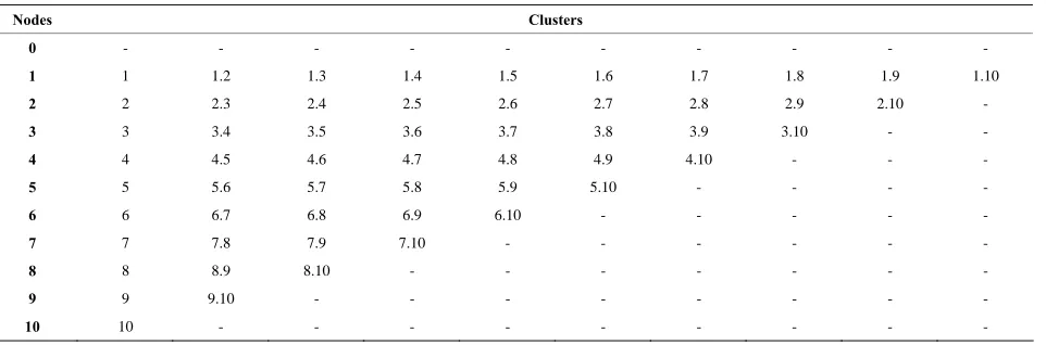
routes covering i as well as the largest possible number of other client nodes in the upper level of order <. As an example, consider the case of 10 client nodes demanding 50 units and a vehicle capacity of 100 units. Table 1 shows the distances among nodes, being 0 the storage site from which departs the vehicle. Table 2 shows the result of the first stage of the procedure. Notice that, since the capacity of the vehicle is 100 and each client node demands 50, a route that clusters some clients to-gether can only consist of two of them. So, for instance the group corresponding to node 9 includes only two possible clusters, {9} and {9,10}, because all other nodes have already been assigned to other clusters. Cluster {9,10} is of a higher order than {9} because it includes two clients instead of just one node.
3.2. Second Stage
At this point a Genetic Algorithm [24] is applied, de-signed for its use in this problem. An individual is codi-fied in a chromosome constructed in such way as to sat-isfy conditions 2) and 3) and therefore are feasible under problem (2). The coding operates on a lexicographic ba-sis. Each is given a number, starting with i = 1, and following the process according to order <. So, take all the clusters ordered according to 1. This order can
Table 1. Distances—Case: 10 nodes / Demand per node: 50 units / Vehicle capacity: 100 units.
Nodes 0 1 2 3 4 5 6 7 8 9 10
0 0.00 5.00 14.14 7.07 11.18 15.81 14.14 5.00 11.18 11.18 18.03
1 5.00 0.00 11.18 11.18 15.81 20.62 18.03 10.00 7.07 10.00 22.36
2 14.14 11.18 0.00 15.81 25.00 25.50 20.00 18.03 5.00 20.62 32.02
3 7.07 11.18 15.81 0.00 11.18 10.00 7.07 5.00 15.00 18.03 18.03
4 11.18 15.81 25.00 11.18 0.00 11.18 15.00 7.07 22.36 15.81 7.07
5 15.81 20.62 25.50 10.00 11.18 0.00 7.07 11.18 25.00 25.00 15.00
6 14.14 18.03 20.00 7.07 15.00 7.07 0.00 11.18 20.62 25.00 20.62
7 5.00 10.00 18.03 5.00 7.07 11.18 11.18 0.00 15.81 14.14 14.14
8 11.18 7.07 5.00 15.00 22.36 25.00 20.62 15.81 0.00 15.81 29.15
9 11.18 10.00 20.62 18.03 15.81 25.00 25.00 14.14 15.81 0.00 20.00
10 18.03 22.36 32.02 18.03 7.07 15.00 20.62 14.14 29.15 20.00 0.00
Table 2. Clusters—Case: 10 nodes / Demand per node: 50 units / Vehicle capacity: 100 units.
Nodes Clusters
0 - - -
1 1 1.2 1.3 1.4 1.5 1.6 1.7 1.8 1.9 1.10
2 2 2.3 2.4 2.5 2.6 2.7 2.8 2.9 2.10 -
3 3 3.4 3.5 3.6 3.7 3.8 3.9 3.10 - -
4 4 4.5 4.6 4.7 4.8 4.9 4.10 - - -
5 5 5.6 5.7 5.8 5.9 5.10 - - - -
6 6 6.7 6.8 6.9 6.10 - - -
7 7 7.8 7.9 7.10 - - -
8 8 8.9 8.10 - - -
9 9 9.10 - - -
10 10 - - -
j
order j is applied to a subset of S
i
i
obtained by elimi-nating (“filtered out”) all the clusters that include nodes already present in clusters corresponding to genes i = 1,···, j – 1. The new ordering is denoted . Then the j-th gene in the chromosome is the rank in of the cluster that is chosen. If for a given i the domain obtained is (because all possible nodes belong to clusters cor-responding to genes 1 to i – 1), any number between 1 and Si can be assigned to the i-th gene. In this way, a chromosome is defined, each corresponding to a feasible solution to problem (2). The Genetic Algorithm seeks to find the optimal one.
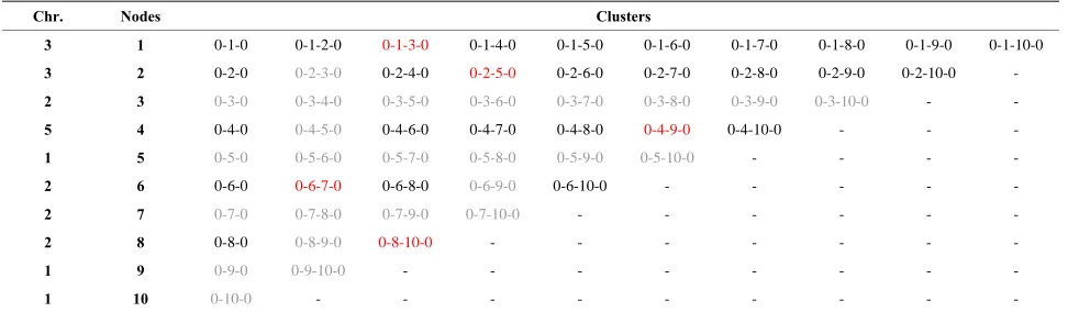
We can see some examples of how chromosomes en-code clusters in Table 3, (3-3-2-1-4-2-3-2-1-1) and Ta-ble 4 (5-2-1-5-1-4-2-2-1-1): all routes start and end at node 0 and go through two client nodes; in gray we see the filtered out clusters and in red the selection. Consider for instance the second gene in Table 3: it has to discard (written in gray) all routes that go through node 3, since it has already been assigned to the first gene. Number 3 assigned to this gene indicate that the route selected is the third in the list of non-filtered routes. On the other hand, a number assigned to a gene with a row with all routes filtered out does not have any effect. The initial
population consists of individuals whose chromosomes are constituted by genes selected at random. Once estab-lished a chromosome, it is decoded and evaluated. This evaluation is performed according to problem (2). For the computation of each cluster we use Lin-Kerninghan’s algorithm that yields the minimal distance among its nodes. The following operators have been chosen in the light of some previous evaluations. The cross-over op-erator is the two-point one (Table 5, Parent 1: 3-3- 2-_-_-_-_-2-1-1, Parent 2: _-_-_-5-1-4-2-_-_-_, Offspring: 3-3-2-5-1-4-2-2-1-1) and the mutation operator alters gene values at 10% of the chromosome (Mutation (Table 6, Offspring*: 3-3-2-5-1-2-2-2-1-1)). Finally, the selec-tion is by ranking.
The Genetic Algorithm runs until the solution gets sta-bilized. These tests were implemented with a C++ pro-gram running on a 3.00 GHZ CPU with a 2.00 GB RAM. The parameters of the experiments were as follows. The size of the population: 100; the cross-over probability: 0.70 and the probability of mutation: 0.01.
[image:3.595.63.544.279.438.2]Table 3. Example of a chromosome ( 3-3-2-1-4-2-3-2-1-1) that will act as parent 1 in the cross-over of Table 5.
Chr. Nodes Clusters
3 1 0-1-0 0-1-2-0 0-1-3-0 0-1-4-0 0-1-5-0 0-1-6-0 0-1-7-0 0-1-8-0 0-1-9-0 0-1-10-0
3 2 0-2-0 0-2-3-0 0-2-4-0 0-2-5-0 0-2-6-0 0-2-7-0 0-2-8-0 0-2-9-0 0-2-10-0 -
2 3 0-3-0 0-3-4-0 0-3-5-0 0-3-6-0 0-3-7-0 0-3-8-0 0-3-9-0 0-3-10-0 - -
1 4 0-4-0 0-4-5-0 0-4-6-0 0-4-7-0 0-4-8-0 0-4-9-0 0-4-10-0 - - -
4 5 0-5-0 0-5-6-0 0-5-7-0 0-5-8-0 0-5-9-0 0-5-10-0 - - - -
2 6 0-6-0 0-6-7-0 0-6-8-0 0-6-9-0 0-6-10-0 - - -
3 7 0-7-0 0-7-8-0 0-7-9-0 0-7-10-0 - - -
2 8 0-8-0 0-8-9-0 0-8-10-0 - - -
1 9 0-9-0 0-9-10-0 - - -
[image:4.595.58.540.264.402.2]1 10 0-10-0 - - -
Table 4. Example of a chromosome ( 5-2-1-5-1-4-2-2-1-1) that will act as parent 2 in the cross-over of Table 5.
Chr. Nodes Clusters
5 1 0-1-0 0-1-2-0 0-1-3-0 0-1-4-0 0-1-5-0 0-1-6-0 0-1-7-0 0-1-8-0 0-1-9-0 0-1-10-0
2 2 0-2-0 0-2-3-0 0-2-4-0 0-2-5-0 0-2-6-0 0-2-7-0 0-2-8-0 0-2-9-0 0-2-10-0 -
1 3 0-3-0 0-3-4-0 0-3-5-0 0-3-6-0 0-3-7-0 0-3-8-0 0-3-9-0 0-3-10-0 - -
5 4 0-4-0 0-4-5-0 0-4-6-0 0-4-7-0 0-4-8-0 0-4-9-0 0-4-10-0 - - -
1 5 0-5-0 0-5-6-0 0-5-7-0 0-5-8-0 0-5-9-0 0-5-10-0 - - - -
4 6 0-6-0 0-6-7-0 0-6-8-0 0-6-9-0 0-6-10-0 - - -
2 7 0-7-0 0-7-8-0 0-7-9-0 0-7-10-0 - - -
2 8 0-8-0 0-8-9-0 0-8-10-0 - - -
1 9 0-9-0 0-9-10-0 - - -
1 10 0-10-0 - - -
Table 5. Cross-over (offspring: 3-3-2-5-1-4-2-2-1-1).
Chr. Nodes Clusters
3 1 0-1-0 0-1-2-0 0-1-3-0 0-1-4-0 0-1-5-0 0-1-6-0 0-1-7-0 0-1-8-0 0-1-9-0 0-1-10-0
3 2 0-2-0 0-2-3-0 0-2-4-0 0-2-5-0 0-2-6-0 0-2-7-0 0-2-8-0 0-2-9-0 0-2-10-0 -
2 3 0-3-0 0-3-4-0 0-3-5-0 0-3-6-0 0-3-7-0 0-3-8-0 0-3-9-0 0-3-10-0 - -
5 4 0-4-0 0-4-5-0 0-4-6-0 0-4-7-0 0-4-8-0 0-4-9-0 0-4-10-0 - - -
1 5 0-5-0 0-5-6-0 0-5-7-0 0-5-8-0 0-5-9-0 0-5-10-0 - - - -
4 6 0-6-0 0-6-7-0 0-6-8-0 0-6-9-0 0-6-10-0 - - -
2 7 0-7-0 0-7-8-0 0-7-9-0 0-7-10-0 - - -
2 8 0-8-0 0-8-9-0 0-8-10-0 - - -
1 9 0-9-0 0-9-10-0 - - -
1 10 0-10-0 - - -
Table 6. Mutation (offspring*: 3-3-2-5-1-4-2-2-1-1).
Chr. Nodes Clusters
3 1 0-1-0 0-1-2-0 0-1-3-0 0-1-4-0 0-1-5-0 0-1-6-0 0-1-7-0 0-1-8-0 0-1-9-0 0-1-10-0
3 2 0-2-0 0-2-3-0 0-2-4-0 0-2-5-0 0-2-6-0 0-2-7-0 0-2-8-0 0-2-9-0 0-2-10-0 -
2 3 0-3-0 0-3-4-0 0-3-5-0 0-3-6-0 0-3-7-0 0-3-8-0 0-3-9-0 0-3-10-0 - -
5 4 0-4-0 0-4-5-0 0-4-6-0 0-4-7-0 0-4-8-0 0-4-9-0 0-4-10-0 - - -
1 5 0-5-0 0-5-6-0 0-5-7-0 0-5-8-0 0-5-9-0 0-5-10-0 - - - -
2 6 0-6-0 0-6-7-0 0-6-8-0 0-6-9-0 0-6-10-0 - - -
2 7 0-7-0 0-7-8-0 0-7-9-0 0-7-10-0 - - -
2 8 0-8-0 0-8-9-0 0-8-10-0 - - -
1 9 0-9-0 0-9-10-0 - - -
[image:4.595.59.542.432.566.2] [image:4.595.56.542.593.735.2]0 (storage site) 1
4
7 9
10
2
3
5
6 8
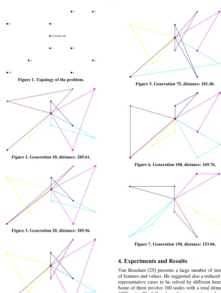
Figure 1. Topology of the problem.
Figure 2. Generation 10, distance: 205.61.
Figure 3. Generation 20, distance: 205.56.
Figure 4. Generation 45, distance: 201.65.
routes generated in several generations and the minimal total distance covered by the selected routes.
Figure 5. Generation 75, distance: 201.40.
[image:5.595.69.516.65.657.2]Figure 6. Generation 100, distance: 169.76.
Figure 7. Generation 150, distance: 153.06.
4. Experiments and Results
Table 7. Results for the problems of Van Breedam [25,26].
Best Solution Found Instance Best Known Solution
Best Solution Evaluations Success (%) Average Solution ∆ (%) Average Time (min)
Bre-1 1106.00 1157.00 395347.12 ± 125177.89 42.00 1169.02 ± 14.76 –4.61 25.16
Bre-2 1506.00 1587.00 374623.02 ± 25544.61 18.00 1595.75 ± 16.91 –5.38 24.11
Bre-3 1751.00 1751.00 121640.67 ± 25684.27 100.00 1751.00 ± 0.00 0.00 11.20
Bre-4 1470.00 1470.00 287936.32 ±14739.13 100.00 1470.00 ± 0.00 0.00 19.68
Bre-5 950.00 985.00 326733.84 ± 112846.01 76.00 994.12 ± 11.49 –3.68 21.66
Bre-6 969.00 979.00 523967.47 ± 162502.07 62.00 982.43 ± 6.59 –1.03 31.72
Bre-9 1690.00 1790.00 657281.22 ± 21838.39 17.00 1797.93 ± 8.03 –5.92 38.52
Bre-10 1026.00 1026.00 871531.96 ± 326830.70. 52.00 1035.85 ± 9.42 0.00 49.45
Bre-11 1128.00 1187.00 1342635.29 ± 543765.65 100.00 1187.00 ± 0.00 –5.23 73.47
units in Bre-5 and Bre-6. Problems Bre-7 and Bre-8 have not been considered because they involve both deliveries and pickups. In most of these problems a single type of good is assumed. Exceptions are problems Bre-9 to Bre-11, in which demands are heterogeneous. Finally Bre-12 to Bre-15 are problems involving time windows, and therefore are not included in our experiments. Table 7 presents the results of our tests. The best known solu-tion, drawn from [25,26], is presented as well as infor-mation on the solutions under our procedure (best solu-tion, average evaluasolu-tion, success, mean solusolu-tion, average running times and percentage of difference with the best known solution). With respect to the processing time, some instances took only minutes while others required hours, although in average the best solutions took not much longer than an hour to be found.
5. Conclusion
We presented a new algorithm for the CVRP (Capaci-tated Vehicle Routing Problem), distinguishing between the standard and its alternative formulation. The details of the procedure were described and the comparison with results in the literature has been presented. While the outcomes are similar to them, their running times are not. In experiments not discussed here we noticed that prob-lems that exceed 100 nodes the processing time is much longer, due to the demands of the first stage of the algo-rithm. We plan to add further search filters at the optimi-zation stage as well as to try with other meta-heuristics to run on the alternative model.
6. Acknowledgements
This work has been supported by several funding sources. The authors are in particular thankful to the National Research Council of Argentina (CONICET) as well as to the Universidad Nacional del Sur project PGI 24/J056.
REFERENCES
[1] D. Ambrosino and A. Sciomachen, “A Food Distribution Network Problem: A Case Study,” IMA Journal of Man-agement Mathematics, Vol. 18, No. 1, 2007, pp. 33-53.
doi:10.1093/imaman/dpl012
[2] L. D. Bodin and B. L. Golden, “Classification in Vehicle Routing and Scheduling,” Networks, Vol. 11. No. 2, 1981, pp. 97-108. doi:10.1002/net.3230110204
[3] S. N. Kumar and R. Panneerselvam, “A Survey on the Vehicle Routing Problem and Its Variants,” Intelligent Information Management, Vol. 4, No. 3, 2012, pp. 66-74.
doi:10.4236/iim.2012.43010
[4] G. Laporte and I. H. Osman, “Routing Problems: A Bib- liography,” Annals of Operations Research, Vol. 61, No. 1, 1995, pp. 227-262. doi:10.1007/BF02098290
[5] E. Mota, V. Campos and A. Corbéran, “A New Metaheu-ristic for the Vehicle Routing Problem with Split De-mands,” In: J. van Hemert and C. Cotta, Eds., Evolution-ary Computation in Combinatorial Optimization, Lecture Notes in Computer Science Vol. 4446, Springer-Verlag, Berlin, 2007, pp. 121-129.
doi:10.1007/978-3-540-71615-0_11
[6] R. Tavakkoli-Moghaddam, N. Safaei, M. Kah and M. Rabbani, “A New Capacitated Vehicle Routing Problem with Split Service for Minimizing Fleet Cost by Simu-lated Annealing,” Journal of the Franklin Institute, Vol. 344, No. 5, 2007, pp. 406-425.
doi:10.1016/j.jfranklin.2005.12.002
[7] J. M. Belenguer, E. Benavent, N. Labadi, C. Prins and M. Reghioui, “Split Delivery Capacitated Arc-Routing Prob-lem: Lower Bound and Metaheuristic,” Transportation Science, Vol. 44, No. 2, 2010, pp. 206-220.
doi:10.1287/trsc.1090.0305
[8] S. R. Thangiah, A. Fergany and S. Awan, “Real-Time Split-Delivery Pickup and Delivery Time Window Prob-lems with Transfers,” Central European Journal of Op-erations Research, Vol. 15, No. 4, 2007, pp. 329-349.
doi:10.1007/s10100-007-0035-x
New Optimization Algorithm for the Vehicle Routing Problem with Time Windows,” Operations Research, Vol. 40, No. 2, 1002, pp. 342-354. doi:10.1287/opre.40.2.342
[10] C. G. Lee, M. A. Epelman, C. White and Y. A. Bozer, “A Shortest Path Approach to the Multiple-Vehicle Routing Problem with Split Pick-Ups,” Transportation Research, Vol. 40, No. 4, 2006, pp. 265-284.
doi:10.1016/j.trb.2004.11.004
[11] P. Belfiore and H. T. I. Yoshizaki, “Scatter Search for a Real-Life Heterogeneous Fleet Vehicle Routing Problem with Time Windows and Split Deliveries in Brazil,” Euro-pean Journal of Operational Research, Vol. 199, No. 3, 2009, pp. 750-758. doi:10.1016/j.ejor.2008.08.003
[12] J. H. Wilck IV and T. M. Cavalier, “A Construction Heu-ristic for the Split Delivery Vehicle Routing,” American Journal of Operations Research, Vol. 2, No. 2, 2012, pp. 153-162. doi:10.4236/ajor.2012.22018
[13] Y. Nagao and H. Nagamochi, “A DP-Based Heuristic Algorithm for the Discrete Split Delivery Vehicle Rout-ing Problem,” Journal of Advanced Mechanical Design,
Systems, and Manufacturing, Vol. 1, No. 2, 2007, pp. 217-226. doi:10.1299/jamdsm.1.217
[14] Y. Yu, H. Chen and F. Chu, “A New Model and Hybrid Approach for Large Scale Inventory Routing Problems,”
European Journal of Operational Research, Vol. 189, No. 3, 2008, pp. 1022-1040. doi:10.1016/j.ejor.2007.02.061
[15] M. A. Nowak, O. Ergun and C. C. White, “An Empirical Study on the Benefit of Split Loads with the Pickup and Delivery Problem,” European Journal of Operational Research, Vol. 198, No. 3, 2009, pp. 734-740.
doi:10.1016/j.ejor.2008.09.041
[16] Z. Shen, M. M. Dessouky and F. Ordóñez, “A Two-Stage Vehicle Routing Model for Large-Scale Bioterrorism Emer- gencies,” Networks, Vol. 54, No. 4, 2009, pp. 255-269.
doi:10.1002/net.20337
[17] L. Moreno, M. P. de Aragao and E. Uchoa, “Improved Lower Bounds for the Split Delivery Vehicle Routing Problem,” Operations Research Letters, Vol. 38, No. 4, 2010, pp. 302-306. doi:10.1016/j.orl.2010.04.008
[18] M.-C. Bolduc, G. Laporte, J. Renaud and F. F. Boctor, “A Tabu Search Heuristic for the Split Delivery Vehicle Rout-
ing Problem with Production and Demand Calendars,”
European Journal of Operational Research, Vol. 202, No. 1, 2010, pp. 122-130. doi:10.1016/j.ejor.2009.05.008
[19] U. Derigs, B. Li and U. Vogel, “Local Search-Based Metaheuristics for the Split Delivery Vehicle Routing Problem,” Journal of the Operational Research Society, Vol. 61, No. 9, 2009, pp. 1356-1364.
doi:10.1057/jors.2009.100
[20] M. Jin, K. Liu and R. O. Bowden, “A Two-Stage Algo-rithm with Valid Inequalities for the Split Delivery Vehi-cle Routing Problem,” International Journal of Produc-tion Economics, Vol. 105, No. 1, 2007, pp. 228-242.
doi:10.1016/j.ijpe.2006.04.014
[21] R. E. Aleman and R. R. Hill, “A Tabu Search with Vo- cabulary Building Approach for the Vehicle Routing Prob- lem with Split Demands,” International Journal of Meta- heuristics, Vol. 1, No. 1, 2010, pp. 55-80.
doi:10.1504/IJMHEUR.2010.033123
[22] R. E. Aleman, X. Zhang and R. R. Hill, “An Adaptive Memory Algorithm for the Split Delivery Vehicle Rout-ing Problem,” Journal of Heuristics, Vol. 16, No. 3, 2010, pp. 441-473. doi:10.1007/s10732-008-9101-3
[23] S. Basu, “Tabu Search Implementation on Traveling Sales- man Problem and Its Variations: A Literature Survey,”
American Journal of Operations Research, Vol. 2, No. 2, 2012, pp. 163-173. doi:10.4236/ajor.2012.22019
[24] D. Goldberg, “Genetic Algorithms in Search, Optimiza-tion, and Machine Learning,” Addison-Wesley Longman Publishing Co., Inc., Boston, 1989.
[25] A. Van Breedam, “An Analysis of the Behavior of Heu-ristics for the Vehicle Routing Problem for a Selection of Problems with Vehicle Related, Customer-Related, and Time-Related Constraints,” Ph.D. Thesis, University of Antwerp—RUCA, Antwerpen, 1994.
[26] E. Alba and B. Dorronsoro, “A Hybrid Cellular Genetic Algorithm for the Capacitated Vehicle Routing Problem,” In: Engineering Evolutionary Intelligent Systems, Chap-ter 13, Studies in Computational Intelligence, Springer- Verlag, Heidelberg, 2008, pp. 379-422.
![Table 7. Results for the problems of Van Breedam [25,26].](https://thumb-us.123doks.com/thumbv2/123dok_us/40278.503840/6.595.55.542.101.291/table-results-problems-van-breedam.webp)
