Control strategy for variable gait using variable knee stiffness in a bipedal robot model

University of Twente

EEMCS / Electrical Engineering

Robotics and Mechatronics

Control Strategy for Variable Gait using Variable Knee

Stiffness in a Bipedal Robot Model

W. (Wesley) Roozing

MSc Report

Committee:

Prof.dr.ir. S. Stramigioli Dr. R. Carloni E. Barrett, MSc Prof.dr.ir. H. van der Kooij

January 2014

John Cleese, The Ministry of Silly Walks

Contents

1 Introduction

4

2 Paper 1: Variable Bipedal Walking Gait with Variable Leg Stiffness

5

3 Paper 2: Bipedal Walking Gait with Segmented Legs and Variable Stiffness

Knees

14

4 Conclusions

25

5 Recommendations

26

A Appendix: 20-sim models

27

A.1 Main model . . . 27

A.2 Controller . . . 29

A.3 Variable Stiffness Actuator (VSA) model . . . 30

1

Introduction

The work described in this master thesis investigates the control of bipedal walking robots

based on the principle of passive dynamic walking. Inspired by the high performance of human

walking, which combines high robustness with high energy efficiency, the goal has been to use

variable leg stiffness to obtain variable walking gait while combining these two aspects. In

contrast, most existing systems are either energy efficient or robust.

The thesis consists mainly of two papers; the first investigates the use of variable leg stiffness

to obtain variable gait on the Spring-Loaded Inverted Pendulum (SLIP) model. The parameter

space in which gaits of a desired velocity exist is first explored and a normalised unique

descrip-tion of a SLIP gait is developed. Based on the control of variable leg stiffness, a gait switching

strategy is proposed that controls the system from one limit cycle walking gait to another in

order to change the walking speed. The strategy is shown to be able to control the system to

another gait within a limited number of steps, after which control action converges to zero.

The second paper investigates the Segmented Spring-Loaded Inverted Pendulum (S-SLIP)

model, which is different from the SLIP model in that it has legs with torsional stiffness knees,

which is more realistic as compared to existing robot designs, which use knees and leg retraction

to avoid food scuffing. It is shown that the S-SLIP model exhibits walking gait, and a control

strategy is developed that is able to stabilise the system after a disturbance. The gait switching

strategy is applied to this model and it is shown that the system can be controlled from one

limit cycle walking gait to another.

Furthermore, a realistic bipedal robot model is designed that uses Variable Stiffness

Ac-tuators (VSAs) to control the knee stiffness. The control is based on the strategy developed

for the S-SLIP model, and is extended with additional components to facilitate hip swing and

leg retraction, which arise due to the additional dynamics of this model. A reference gait is

obtained by using this model with constant leg stiffness. The variable knee stiffness is then

used to stabilise the system into this gait and to inject energy losses generated by foot impacts.

It is shown that this results in a stable limit cycle walking gait. The thesis concludes with a

discussion of results obtained and recommendations for future work.

2

Paper 1: Variable Bipedal Walking Gait with Variable Leg

Stiffness

Submitted to ICRA 2014.

Abstract

– The Spring-Loaded Inverted Pendulum (SLIP) model has been shown to exhibit

many properties of human walking, and therefore has been the starting point for studies on

robust, energy-efficient walking for robots. We address the problem of online gait variation on

the SLIP model by control of the leg stiffness and adjustment of the angle-of-attack in order to

switch between gaits and thus regulate walking speeds. We show that it is possible to uniquely

describe SLIP limit cycle gaits in fully normalised form. Using that description, we propose

both an instantaneous switching method and an interpolation method with an optimisation step

to switch between limit cycle SLIP gaits. Using simulations, we show that it is then possible to

transition between them online, after which the system converges back to zero-input limit cycle

walking.

Variable Bipedal Walking Gait with Variable Leg Stiffness

W. Roozing, L.C. Visser, and R. Carloni

Abstract— The Spring-Loaded Inverted Pendulum (SLIP) model has been shown to exhibit many properties of human walking, and therefore has been the starting point for studies on robust, energy-efficient walking for robots. We address the problem of online gait variation on the SLIP model by control of the leg stiffness and adjustment of the angle-of-attack in order to switch between gaits and thus regulate walking speeds. We show that it is possible to uniquely describe SLIP limit cycle gaits in fully normalised form. Using that description, we propose both an instantaneous switching method and an interpolation method with an optimisation step to switch between limit cycle SLIP gaits. Using simulations, we show that it is then possible to transition between them online, after which the system converges back to zero-input limit cycle walking.

I. INTRODUCTION

This work is inspired by the high performance of human walking, which combines high robustness with high energy efficiency. In contrast, most existing legged robotic systems show either high robustness or energy efficiency.

Passive dynamic walking can be realised by designing mechanics such that it has a walking gait as dynamic mode [1]. However, while designs based on the principle of passive dynamic walking show high energy efficiency, they are not very robust against external disturbances. Other, highly controlled systems show high robustness at the exchange of energy efficiency [2]. Combining these two aspects has proven difficult. Furthermore, these robots rely on compass gaits, using either stiff legs or locking the knee during walking, which does not resemble human legs.

It has been shown that human walking on flat terrain can be accurately modeled by an inverted passive mass-spring system. The Spring-Loaded Inverted Pendulum (SLIP) model shows walking dynamics strongly comparable to human walking in terms of hip trajectory, single- and double-support phases and ground contact forces [3]. It exhibits self-stable walking and running gait for a relatively large range of system parameters. It can demonstrate walking with different forward velocities as well as running [3], [4]. Although the SLIP model exhibits self-stable walking gait for large ranges of parameters on its own, it has been shown that the basin of attraction can be enlarged by control of a variable leg stiffness [5]. The Variable SLIP (V-SLIP) model significantly increases robustness against external disturbances and, after a disturbance, is able to restabilise the system into its original gait by injecting or removing energy appropriately.

It is very desirable to be able to change the forward velocity of legged robots, for example slowing down to save

W. Roozing and R. Carloni are with the Robotics And Mechatronics group, MIRA Institute, University of Twente, The Netherlands. E-mail: [email protected], [email protected]

energy, or speeding up to travel large distances quickly. In [6], it was shown that it is possible to change gait on the SLIP model by controlling the angle-of-attack. However, the method relies on imposing constant system energy, thus significantly reducing achievable velocities by injecting or removing energy in the system. In [7], the authors propose velocity control of a four-link walking model with stiff legs by changing step length and the frequency of the hip actuation. By placing their robot on a slope, they negate the loss of energy due to foot impacts and propose a velocity control strategy by controlling the slope. The work done in [8] shows in simulation and experiment that it is possible to change velocity by changing step length and joint stiffnesses. They use variable stiffness actuators in each joint, but lock the stance leg knee to support the robot. A stiff-legged walker is also used in [9], but the authors vary the pitch of a torso to induce different walking speeds. These works rely on compass gaits, using either stiff legs or locked knees during stance.

The problem of online gait variation is addressed in this work by the design of a control strategy for the V-SLIP model that allows to switch between limit cycle gaits during walking by actively controlling the leg stiffness and angle-of-attack. We propose an optimisation criterion that aligns the two gaits and then switches between them by changing control references and system parameters appropriately, after which the system converges back to zero-input limit cycle walking. Energy is injected or removed from the system appropriately to accommodate the new gait.

The remainder of this paper is outlined as follows. Section II describes the SLIP model. Also, a normalised notation of SLIP limit cycle gaits is introduced. Section III outlines the control strategy to control the V-SLIP system and switch between limit cycle gaits. Section V contains simulation results of the proposed method. Lastly, Section VI concludes on the work and proposes directions for future efforts.

II. THE SPRING-LOADED INVERTED PENDULUM (SLIP) MODEL

A. SLIP Dynamics

The bipedal Spring-Loaded Inverted Pendulum (SLIP) model is shown in Fig. 1. It consists of a hip point massm, which connects two massless telescopic legs. The legs consist of springs with rest lengthL0 and stiffnessesk1=k2=k0. Given properly chosen initial conditions, the SLIP model shows stable passive walking gaits [3], [4].

y

x m

k1 k2

c2 c1

Fig. 1. The SLIP model consists of a hip point massm, with two massless telescopic springs with stiffnesses k1 =k2 =k0 as legs. The model is

shown during double-support phase, with both legs touching the ground at contact pointsc1andc2.

the tangent space toQ atq. The system state is then given as x := (q,p), with the momentum p := (px, py) = Mq˙

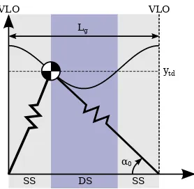
and the mass matrix M = diag(m, m). A single step is defined as a trajectoryq(t)_{∈ Q}that starts with the system in Vertical Leg Orientation (VLO), where the hip mass is exactly above the supporting leg. The step ends when the system again reaches VLO (Fig. 2), and the role of the legs is then exchanged. We define the gait length Lg :=x(T),

i.e. the distance travelled after one step, whereT is the gait time period.

During a single step, two phases must be distinguished – single-support (SS) and double-support (DS), during which one and two legs are in touch with the ground respectively. The transition from single- to double-support occurs when the mass reaches the touch-down heightytdassociated with the angle-of-attackα0and the swing leg touches the ground (Fig. 2):

y=ytd:=L0sin(α0) (1)

The location of the leading contact pointc2is then calculated as (Fig. 1):

c2=x+L0cos(α0) (2)

Similarly, the transition from double- to single-support oc-curs when either leg reaches its rest length:

q

(x₋ci)2+y2_{=L0, i∈ {1,2} (3)}

At transition to single-support, the swing leg disappears and reappears at the subsequent instance of touch-down, which is possible because the leg is massless. In the nominal case, only the trailing leg reaches its rest length and contact c2 is relabeled asc1 to correspond to the notation used during single-support phase. We can now define two subsets of Q

which correspond to the single- and double-support phases respectively:

QSS ={q∈ Q |y > ytd, y < L0}

QDS ={q∈ Q |y < ytd, y >0}

(4)

wherey < L0andy >0are included to avoid the remaining

cases, i.e. lift-off and fall respectively. Note that for a walking

ytd

Lg

VLO VLO

α0

DS

SS SS

Fig. 2. A single step of the SLIP model, shown at the moment of touchdown. The step starts and ends at VLO and has lengthLg. Note that at touchdown, the swing leg is at exactlyα0with the ground and has length

L0. At touchdown, the SLIP model goes into double-support (DS) phase,

shown by the touch-down heightytd, and returns into single-support (SS) phase when the hip again crossesytdand the trailing leg reaches length L0.

gaitq_{∈ Q}SS∪ QDS.1

2) System Dynamics: To derive the dynamic equations for the system, we use the Hamiltonian approach. The kinetic energy function is defined as K = 1

2p

T_M−1_{p and the} potential energy function as

V =mgy+1

2k0(L0−L1)

2

+1

2k0(L0−L2)

2

where Li =

q

(x₋ci)2+y2 _{and g is the gravitational} acceleration. During single-support phase, we set L2_≡L0, i.e. the swing leg is uncompressed and it exerts no force. The dynamic equations are then defined by the Hamiltonian energy functionH =K+V as

d dt

q p

=

0 I

−I 0

"δH δq δH δp #

(5)

Note that a solutionq(t)of (5) is of classC2_{, due to the} non-differentiability of the leg forces at the moment of transition between the single- and double-support phases.

B. Limit Cycle Gaits for the SLIP Model

It was shown [4] that, given the proper system param-eters and initial conditions, the dynamics described by (5) exhibit autonomous stable walking gait. A limit cycle gait is a periodic walking gait which returns to the same state periodically. From this point on, we refer to limit cycle gaits of the SLIP model asnatural gaits.

In our description of natural gaits we use the state at VLO as initial conditions, i.e.x0= (q,p)0= (x, y, px, py)0, and, during walking in natural gait, the system returns to this state at every VLO. Since we can take at VLOx_≡0, a natural

gait can then be fully described as

Σ = (α0, k0, L0, m, y0, px,0, py,0) (6)

1_{Lift-off is also possible whileq∈ QSS∪ QDS. We take care of this in}

simulation by checkingL1≤L0∨L2≤L0, i.e. there is always at least

Note that it is not possible to use the total system energyH to uniquely describe a natural gait, because energy can be stored in either potential or kinetic energy.

C. A Normalised Notation of SLIP Limit Cycle Gaits

k0andH can be normalised, such that SLIP models with different parameters can be compared easily:

˜

k=k0L0

mg H˜ =

H

L0mg (7)

If we normalisexas x˜:= (˜q,p˜) = (˜x,y,˜ px,˜ py˜ )with

˜

x= x

L0 y˜=

y

L0 px˜ =

px

m√L0g py˜ =

py

m√L0g (8)

and use (7), we obtain a fully normalised unique description

˜

Σof a natural gait:

˜

Σ =α0,˜k,y0,˜ px,0,˜ py,0˜ (9)

The gait trajectory can then be found by solving (5) for _Σ˜_.

Using this description, equal gaits on different SLIP systems now result in the same normalised state trajectory x˜(t) = (˜q(t),p˜(t)). Similarly topx,˜ py˜ , the velocities are normalised as

˙˜

x=√_L0gx˙ y˙˜=√_L0gy˙ (10)

Note that the normalisationx˙˜is the Froude numberF r [8], [9], used to compare the relative walking speeds of systems with different leg lengths.

III. CONTROL DESIGN

By actively controlling the leg stiffness of the SLIP model, the robustness of the system to external disturbances can be significantly increased and, after a disturbance, the system can be stabilised into its original gait by injecting or removing energy appropriately [5]. The extended model, called Variable-SLIP (V-SLIP), replaces the constant stiffness legs by variable stiffness legs.

We use the ability to change the leg stiffness to transition between gaits. The rationale is as follows. By considering a gait switch as a disturbance to the system which has to be rejected, the system can be controlled into any gait which is within the basin of attraction of the closed loop system. Furthermore, because there are large continuous regions of self-stable natural gaits with different forward velocities [4], the system can change into nearly any gait by using an appropriate transition strategy. In this section, we discuss the leg stiffness control that stabilises the system into a natural gait. The next section will discuss the gait transition strategy. The variable stiffness legs of the V-SLIP model have stiffness ki = k0 +ui, with control inputs ui restricted to subsets Ui = _{ui _{∈ R|}0 < k0 +ui < _∞}, such that the result is physically meaningful. Given a natural SLIP gait_Σ˜ _{and corresponding state trajectoryx˜(t), which}

is a solution of (5), we intend to control the system such that it converges to its natural gait, i.e. a reference x˜◦_(t) such that ui → 0 and ki → k0, i ∈ {1,2}. However, as the system is underactuated during the single-support phase,

these references cannot be tracked exactly, and as the system lags behind the reference this may lead to instability. Because

˜

x was identified as a periodic variable, and required to be monotonically increasing in time, the references may be reparametrised in x˜. Due to the parametrisation in x˜, the gait references are sufficiently described as

˜

y∗(˜x) = ˜yo(˜x) x˙˜∗(˜x) = ˙˜xo(˜x) (11)

However, as a general analytic expression for the spring-loaded pendulum does not exist [10], a Fourier series expan-sion approximation of the numerical solution is used.

To formulate the control strategy, we rewrite Eq. (5) in standard form as

˙

x=f(x) +X

i

gi(x)ui (12)

and then define error functionsh1 andh2 as h1=y−y∗

h2= ˙x₋x˙∗ (13)

The control solution is then given as follows. • Forq∈ QSS:

u1= 1

Lg1Lfh1

−L2fh1−κdLfh1−κph1

u2≡0

(14)

• Forq∈ QDS:

u1 u2

=A−1

−L2

fh1−κdLfh1−κph1

−Lfh2₋κvh2

(15)

with

A=

Lg1Lfh1 Lg2Lfh1

Lg1Lfh2 Lg2Lfh2

(16)

whereL2

fhi,Lfhi and LgiLfhi denote the (repeated) Lie-derivatives ofhi along the vector fields defined in (12) and κd, κp, κvare tunable control parameters. The control inputs (14), (15) ensure that the errorh1 converges asymptotically to zero and that the errorh2 is at least bounded [5].

Remark: Due to the structure of the problem, the system is not fully controllable during the single-support phase. Because the error in y influences touch-down and lift-off events, it is deemed more important. Thus, by design, only h1 is controlled during the single-support phase (Eq. (14)).

Remark:During either single- or double-support, the con-trol inputsu1 and u2 are continuous. However, their conti-nuity is not guaranteed at the moment of phase transition.

IV. GAIT TRANSITION

A. Search of Stable Gaits

Suppose the system described by the SLIP model is in some natural gait and it is commanded to change the velocity. As natural gaits exist for large ranges of parameters, there often exists a range of natural gaits that achieve that velocity. This is shown in Fig. 3. Natural gaits exist for many values of(α0,k˜), and a single set(α0,˜k)can in general achieve a

α0

k ~ ~

xavg Natural gaits for fixed (α0, k)~

~

Values of (α0, k) for

which natural gaits exist

Fig. 3. Average forward velocities x˙˜avg of natural gaits for different values of(α0,˜k). Note that for given(α0,˜k), the average forward velocity

is proportional to the system energy_H.˜

In choosing (α0,k˜), there may be practical design

con-siderations. The range of stiffnesses obtainable in practice is limited, and the range of acceptable angles of attack is limited due to foot slip and energy loss due to high ground impact forces and so forth. Exactly which values of (α0,k˜) are chosen is arbitrary within the ranges of natural gaits. The next sections describe a general method for switching from some given gait_Σ˜_{i to some other given}

gait_Σ˜_{j, independently ofΣ}˜_iandΣ˜_{j. We do, however, make}

a distinction between switching between gaits with equal values of (α0,˜k) (Section IV-C.1) and gaits with different

(α0,˜k)(Section IV-C.2).

B. Optimisation Criterion for Gait Switching

1) Finding Optimal Points: Suppose that two natural gaits

˜

Σi andΣ˜j have been chosen and that we want the system to switch from _Σ˜_{i toΣ}˜_{j. The parametrisation in x˜ of both}

can be used to determine exactly how to transition from one gait to the other. In each gait one point should be considered: The point in_Σ˜_{iat which the switch is executed and the point}

in_Σ˜_{j to switch into. Figure 4 shows example trajectories of} ˜

Σi andΣ˜j. Any pointxi˜ ∈ h

0,Lg,i˜ ion one step ofΣ˜i can be associated with any pointxj˜ ∈h0,Lg,j˜ i on one step of

˜

Σj. A combination of two values(˜xi,opt,xj,opt˜ )should exist that minimises some criterionJ. Intuitively, to minimise the required control input for transition, we propose to transition at a point at which both gaits have approximately equal momentum of the hip mass, that is,pi(xi)≈pj(xj)(Figure 4). However, asmis constant, the velocities x,˙˜ y˙˜are used. As the forward velocity is only controlled during double-support phase, whereas the vertical position is controlled during both single- and double-support, differences inx˙˜are penalised differently than iny˙˜. Thus, both terms are included separately. Additionally, we include the hip height y˜, as it would be beneficial to switch at a point at which the trajectories are close together, such that the resulting error h1 is smaller. We then defineJ(˜xi,xj˜ )as follows:

J(˜xi,xj˜ ) =µ1_kyj˜ (˜xj)₋yi˜(˜xi)_k+

µ2xj˙˜ (˜xj)−xi˙˜(˜xi)+

µ3yj˙˜(˜xj)₋yi˙˜(˜xi)

(17)

By choosing the weightsµ1,2,3, the different aspects of the gait can be emphasised as to achieve a smooth response. The

0

0 y

~

J(x~i, x~j)

xi

~ _x

i,opt ~

J(x~i,opt, x~j,opt)

Gait Σi ~

Lg,i ~

pj(xj)

~ ~

pi(xi)

~ ~ xj ~ _x j,opt ~ Lg,j ~

Gait Σj ~

Fig. 4. Optimisation of the switching point from_Σ˜_{i toΣ}˜_{j. The point} ˜

xiis moved along one step ofΣ˜i, andJ(˜xi,x˜j)is then calculated for all values of˜xjin one step ofΣ˜j. Minimisation ofJfor both these parameters then results in the optimal switching points(˜xi,opt,x˜j,opt). Note that the gaits shown here are spatially separated, while in practice many gaits will overlap, especially those with equal values ofα0.

System

Aligned

xδ,j

~ xj,opt ~ xi,opt ~ Lg,i ~

Sopti,j

~ Lg,j

~

Reference Gait Σ~j Reference Gait Σ~i

Fig. 5. Aligning optimal points of_Σ˜_iandΣ˜_{j, with step lengthsL}˜_g,iand ˜

Lg,jrespectively. The trajectory ofΣ˜jis shifted byx˜δ,j, such that˜xj,opt aligns withx˜i,optat the optimal switching distanceS˜opti,j. The dashed blue lines indicate the natural gait references, the red line indicates an example system response.

criterionJ is then minimised numerically with respect to˜xi andxj˜ to obtain the optimal switching points:

min

˜

xi,˜xj

J(˜xi,xj˜ )_→(˜xi,opt,xj,opt˜ ) (18)

Note that multiple minima may exist, so we search for the global minimum. Due to the use of normalised variables the results are again identical for the same natural gaits on different SLIP systems, and due to symmetry results obtained for_Σ˜_i→Σ˜_{j are also valid forΣ}˜_j→Σ˜_i.

2) Aligning optimal points: As gaits are parametrised as a function of forward distancex˜, we define the gait transitions

in terms of forward distance as well. The switching strategy for a single transition is then summarized as follows. Suppose the system is commanded to switch into gait _Σ˜_{j at a}

distance Si,j

com [m], normalised as S˜comi,j = Si,jcom/L0. We then calculate the optimal switching distance_S˜i,j

opt, which is the first occurrence of the pointxi,opt˜ after this commanded

distance (Fig. 5):

˜

Sopti,j = ˜Si,jcom−S˜i,jcom(mod ˜Lg,i) + ˜xi,opt (19)

If_S˜i,j

opt<S˜i,jcom, we make sure the switching distance is after the commanded distance by calculating_S˜i,j

opt= ˜S

i,j

opt+ ˜Lg,i,

SS DS

State transition within gait Valid gait state transition Invalid gait state transition

Touch-down Touch-down

Lift-off

Lift-off

Gait Σj

SS DS

Gait Σi

Fig. 6. State transitions during limit cycle walking and gait transition. For a single gait, a transition from single-support to double-support and back occurs every step. When switching gaits in single-support, the system transitions to single-support of the new gait, and vice versa. A transition from double-support of gait_Σ˜_{ito single-support of gaitΣ}˜_{j(or vice versa)} is invalid, as that would require foot lift-off at the moment the controller decides to switch gaits, which is infeasible.

can switch into the new gait by changing α0, k˜ and the controller references appropriately.

To ensure the system switches from the optimal point in the step of _Σ˜_{i into the optimal point in the step ofΣ}˜_{j, the}

trajectory of_Σ˜_{j is shifted in such a way that the pointxj,opt˜}

aligns with_S˜i,j

optinx˜. The shiftxδ,j˜ of Σ˜j is calculated as

˜

xδ,j= ˜Sopti,j −xj,opt˜ (20)

By shifting the reference of_Σ˜_{j by xδ,j˜ , the optimal points} (˜xi,opt,xj,opt˜ )are aligned in x˜ (Fig. 5).

C. Switching Strategy

At this point we outline the switching strategy. Although the method is general, we make a distinction between switch-ing between gaits with equal values of(α0,k˜)and gaits with different(α0,˜k). The first case will be shown to be a special case of the second.

Fig. 6 shows the possible states and transitions for some gaits _Σ˜_{i andΣ}˜_{j. For a single gait, a transition from}

single-support to double-single-support and back occurs every step, at touch-down and lift-off respectively (i.e. when y˜ crosses ˜

ytd). However, if the two gaits have different values ofα0, the current hip height may be defined as double-support in

˜

Σi, but as single-support in Σ˜j, i.e. ytd,i˜ > y >˜ ytd,j˜ . This results in an invalid situation if the gait switching is performed instantaneous at that point, as that would require instantaneous foot lift-off at the instant of switching.

However, we do not want to rule out such points entirely by modification of (17). Firstly, because at such points the gait trajectories may be close together in terms of hip height

˜

y resulting in smaller errorh1. Secondly, large variations in α0may cause gaits to be entirely separated in y˜, such as in

Fig. 4, where the entire gait _Σ˜_{j lies under the touch-down}

height of_Σ˜_{i. Therefore, for gaits with equal values of(α0,k}˜₎

instantaneous switching is used, and for gaits with different

(α0,˜k)gait interpolation is used, as outlined below.

1) Instantaneous Switching: As the values of (α0,k˜)

remain constant, we need only to define the controller

references y˜∗(˜x),x˙˜∗(˜x)as:

˜

y∗(˜x) =

˜

yi(˜x) x <˜ S˜opti,j

˜

yj(˜x−xδ,j˜ ) x˜≥S˜opti,j

˙˜

x∗(˜x) =

_˙˜

xi(˜x) x <˜ S˜opti,j

˙˜

xj(˜x−xδ,j˜ ) x˜≥S˜opti,j

(21)

2) Gait Interpolation: To avoid invalid gait transitions (Fig. 6) caused by instantaneously changing the value of α0, we need to ensure the value of α0 is continuous in

˜

x. This way we avoid the invalid state transitions in Fig. 6. We extend (21) with a transition period, during which the two gait references are interpolated, together with the corresponding values ofα0 and˜_k:

˜

y∗(˜x) =

  

˜

yi(˜x) β_≤0

(1₋β)˜yi(˜x) +βyj˜ (˜x₋xδ,j˜ ) 0< β <1 ˜

yj(˜x₋xδ,j˜ ) β_≥1

˙˜

x∗(˜x) =

  

˙˜

xi(˜x) β≤0

(1−β) ˙˜xi(˜x) +βxj˙˜ (˜x−xδ,j˜ ) 0< β <1 ˙˜

xj(˜x) β_≥1

α0=

  

α0,i β≤0

(1−β)α0,i+βα0,j 0< β <1

α0,j β≥1

˜ k=    ˜

ki β_≤0

(1−β)˜ki+βkj˜ 0< β <1

˜

kj β_≥1

(22) where the interpolation factor β is defined as β = (˜x−

˜

Sopti,j)/γ. The parameter γ ≥0 is the transition length. By the definition of the normalised variables, γ effectively is the number of leg lengths inxto interpolate for. Of course,

˜

y∗_,x˙˜∗ _{in (22) converge to (21) asγ→0. The reason we} use (21) for constant(α0,k˜)is that then we let the controller handle the transition as quickly as it can, instead of forcing a transition period of fixed length.

V. RESULTS

To demonstrate the effectiveness of the method for large forward velocity differences, first achievable velocity ranges for selected values of(α0,˜k)that result in symmetric natural

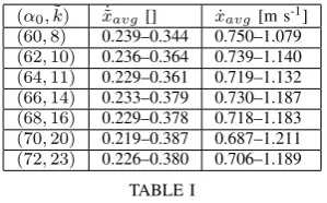
gaits is analysed. Simulations were performed in Mathworks MATLAB R2012b, using the ode45 solver with absolute and relative tolerances of 1e-10. The velocity ranges were found by fixing the vertical velocity at VLO to zero, thus enforcing symmetrical gaits [4], and incrementing the forward velocity at VLO in small steps. The resulting velocity ranges are shown in Table I, wherexavg˙˜ denotes the normalised average forward velocity and xavg˙ denotes the average forward velocity in [m s-1_].

Two simulations are performed. In both cases,m= 80kg and L0 = 1 m. Furthermore, {µ1, µ2, µ3_} = _{15,2,5_}. In the first simulation (Section V-A), a constant value(α0,k˜) = (70,20)is chosen, and two gaits are selected: a slow gait with

average velocity of 0.238 (0.745 m s-1_{, using (8)) and a fast}

gait with average velocity 0.372 (1.164 m s-1_{), an increase of}

(α0,˜k) x˙˜avg [] x˙avg [m s-1] (60,8) 0.239–0.344 0.750–1.079 (62,10) 0.236–0.364 0.739–1.140 (64,11) 0.229–0.361 0.719–1.132 (66,14) 0.233–0.379 0.730–1.187 (68,16) 0.229–0.378 0.718–1.183 (70,20) 0.219–0.387 0.687–1.211 (72,23) 0.226–0.380 0.706–1.189

TABLE I

STABLE FORWARD VELOCITY RANGES FOR SYMMETRICAL GAITS WITH SELECTED VALUES OF(α0,˜k).

0 0.1 0.2 0.3 0.4 0.5

0.92 0.94 0.96 0.98 ˜ x ˜ y

Normalised trajectories + touch−down heights

Gait 1 Gait 2 ytd

Fig. 7. Hip trajectories for a single step of two gaits with(α0,k˜) =

(70,20). The slow gait (1) is double-humped, whereas the faster gait (2) is single-humped. The dotted liney tddenotes the touch-down height, and the solid dots denote the optimal points(˜x1,opt,x˜2,opt).

to moving up and down on one of the vertical bars in Fig. 3, and we use the instantaneous switching method (Section IV-C.1).

In the second (Section V-B), a slow gait with an average velocity of 0.232 (0.725 m s-1_{) and(α0,k}˜_{) = (64,11)and a}

fast gait with an average velocity of 0.372 (1.164 m s-1_{) and} (α0,˜k) = (70,20) are chosen, to demonstrate robustness

against changing the angle of attack. This corresponds to switching from one point on a vertical bar to another point on another bar in Fig. 3. Here we use the gait interpolation withγ= 1.0 (Section IV-C.2).

In both cases, the system starts in the slow gait (gait 1), commanded to change to fast gait (gait 2) at 1.0 m, and then switch back to the slow gait (gait 3 = gait 1) at 5.5 m.

A. Constant (α0,k˜)

Fig. 7 shows the hip trajectory for a single step of both gaits. The first, i.e. slow gait, is double-humped, whereas the faster gait is single-humped. This likely results from the fact that the natural frequency of the hip mass and leg springs remains approximately constant, while the gait period changes. CalculatingJ for these two gaits results in

(˜x1,opt,x2,opt˜ ) = (0.259,0.244), which corresponds approx-imately to the lowest point in both gaits. Of course, for the switch back to the first gait we can use the same values but interchanged. The found values result in optimal switching distances _S˜1,2

opt= 1.306 andS˜

2,3

opt = 5.762 respectively (Eq. (19)).

Fig. 8 shows the resulting hip trajectory with the desired and optimal switching points indicated. The hip returns to a periodic trajectory very quickly. Fig. 9 shows the resulting hip height and forward velocity in time, as well as the natural gait references. It can be seen that because the hip

0 2 4 6 8 10

0.92 0.94 0.96 0.98 ˜ x ˜ y System

Switch gait 1→2

Switch gait 2→3

Fig. 8. Hip trajectory for the transition from slow to fast gait and back for two gaits with constant(α0,˜k). For each pair of vertical dashed lines, the

first indicates the commanded switching distance, and the second indicates the resulting optimal switching distance.

0 2 4 6 8 10

0.92 0.93 0.94 0.95 0.96 0.97 time [s] ˜ y

0 2 4 6 8 10

0.2 0.25 0.3 0.35 0.4 time [s]

˙ ˜x

System Gait 1 reference Gait 2 reference Gait 3 reference

Fig. 9. Hip height and forward velocity over time. The vertical hip motion converges to the new reference within one step. The forward velocity converges in approximately 5 steps.

0 2 4 6 8 10

20 40 60

time [s]

˜k+

˜

u1

,

˜k+

˜

u2 ˜k+ ˜u1 ˜k+ ˜u2 Nominal stiffness

0 2 4 6 8 10

−5 0 5 10

x 10−3

time [s] P o si ti o n er ro r

0 2 4 6 8 10

−0.2 0 0.2 0.4 V el o ci ty er ro r Position error Velocity error

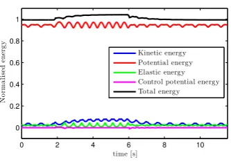
0 2 4 6 8 10 0 0.2 0.4 0.6 0.8 1 time [s] N o rm a li se d en er g y Kinetic energy Potential energy Elastic energy Control potential energy Total energy

Fig. 11. Energy balance. Most of the increase in total energy is used in the kinetic energy of the system. Some of the additional energy results increased vertical motion of the hip.

0 0.1 0.2 0.3 0.4 0.5 0.6

0.85 0.9 0.95 1 ˜ x ˜ y

Normalised trajectories + touch−down heights

Gait 1 Gait 2 ˜

ytd,1

˜

ytd,2

Fig. 12. Hip trajectories for a single step of two gaits with(α0,˜k) =

(64,11)and (70,20)respectively. In contrast with Fig. 7, the gaits are completely separated iny˜and have different touch-down heightsytd,i. The solid dots denote the optimal points(˜x1,opt,x˜2,opt).

height is controlled during both single- and double-support,

˜

y converges to the new reference within a single step. The forward velocity x˙˜ converges to the new reference within approximately 5 steps in both transitions. Fig. 10 shows the control inputs and position and velocity errors. The disturbance that arises from the new references is rejected in approximately one second for the hip height and four seconds for the forward velocity respectively, after which the leg stiffnesses converge back to the nominal value. Fig. 11 shows the energy balance. The energy increases from

˜

H1= 0.993toH2˜ = 1.041after the first switch, which if all

converted to forward kinetic energy would result in a forward velocity ofxavg˙˜ = 0.388 (1.216 m s-1). This shows that not

all added energy is converted into forward momentum but instead into a vertical motion (Fig. 7) and a minor increase in average hip height.

Remark:The small periodic deviations in the inputs (Fig. 10) after convergence arise due to difference between the approximated gait references using Fourier series and the SLIP model dynamics.

B. Gaits with different(α0,˜k)

Fig. 12 shows the hip trajectory for a single step of both gaits. It can be seen that due to the different values ofα0the gaits are completely separated in hip height during the entire step; this also results in a significantly smaller step length for the higher gait. Again calculatingJ for these two gaits, we find (˜x1,opt,x2,opt˜ ) = (0.509,0.259). This corresponds

to approximately the highest point in the first gait and the lowest point in the second gait, arising from the separation of both gaits in terms of hip height. The found values result in

0 1 2 3 4 5 6 7 8 9

0.88 0.9 0.92 0.94 0.96 ˜ x ˜ y System

Switch gait 1→2

Switch gait 2→3

Fig. 13. Hip trajectory for the transition from slow to fast gait and back for two gaits with different(α0,˜k). For each pair of vertical dashed lines, the

first indicates the commanded switching distance, and the second indicates the resulting optimal switching distance.

optimal switching distances_S˜1,2

opt= 1.090 andS˜

2,3

opt= 6.041

respectively.

Fig. 13 shows the resulting hip trajectory with the de-sired and optimal switching points indicated. The trajectory smoothly rises to the new hip height as its shape transforms into that of the second gait. Inspecting the hip height and forward velocity over time (Fig. 14), we see a similar image. The hip oscillation frequency increases as α0 and forward velocity increase. Note how the forward velocity suddenly increases as the system transitions back to the first gait. This is due to α0 decreasing, thus lowering touch-down height, leaving more time for the hip mass to accelerate before touch-down. Fig. 15 shows the corresponding control input and error functions. On a few occasions, the leg stiffness reaches the lower limit. After transition, the leg stiffnesses converge to the new gait’s nominal_k˜_{value. Note that during}

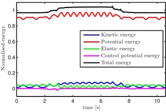
single-support, the stiffness of the swing leg is always equal to˜_{k(Eq. (22)), as u2˜ ≡0in that case (Eq. (14)). The total}

energy again increases to accommodate the faster gait. The increase is converted in both kinetic and potential energy, while the average elastic energy decreases. The latter can be attributed to the higher, more stiff-legged walk of the second gait.

VI. CONCLUSIONS & FUTURE WORK A method was presented that allows to switch between natural gaits by actively controlling the leg stiffness. Using this method it is possible to vary the forward velocity during walking by choosing appropriate natural gaits.

First, a normalised notation of natural gaits was intro-duced. Next a control strategy was proposed that aligns two chosen gaits by minimisation of a criterion, designed such that the transition between the two results in minimal control input. The switch was performed in one of two possible ways; Instantaneous switching for gaits with equal values of the angle of attack and leg stiffness, and gait interpolation with gaits with different values.

0 1 2 3 4 5 6 7 8 9 10 0.88 0.9 0.92 0.94 0.96 time [s] ˜ y

0 1 2 3 4 5 6 7 8 9 10 0.2 0.25 0.3 0.35 0.4 time [s]

˙ ˜x

System Gait 1 reference Gait 2 reference Gait 3 reference

Fig. 14. Hip height and forward velocity over time. The vertical hip motion and forward velocity converge to the new gait in approximately 3 steps.

0 2 4 6 8 10

0 10 20 30 40 time [s]

˜k+

˜

u1

,

˜k+

˜

u2

˜

k_{+ ˜}u₁

˜

k+ ˜u₂

Nominal

0 2 4 6 8 10

−0.02 −0.01 0.01 0.02 time [s] P o si ti o n er ro r

0 2 4 6 8 10 −0.4

0 0.4 V el o ci ty er ro r Position error Velocity error

Fig. 15. Control input and error functions. The disturbances that arise from the new references are rejected, after which the leg stiffness converges to a constant value. Note that during single-support, the stiffness of the swing leg is always equal to_{k, as}˜ _{u˜2≡0in that case (Eq. (14)).}

0 2 4 6 8 10

0 0.2 0.4 0.6 0.8 1 time [s] N o rm a li se d en er g y Kinetic energy Potential energy Elastic energy Control potential energy Total energy

Fig. 16. Energy balance. In the first gait, there is relatively much energy stored as elastic energy, due to the lower leg stiffness. Compared to Fig. 11, there is a significant rise in the potential energy due to the increased hip height of the second gait.

Future work should focus on analysing the robustness of the system during gait transition. Furthermore, it could include a study on more realistic models, such as those including knees and feet, or non-zero leg mass.

REFERENCES

[1] T. McGeer, “Passive dynamic walking,“The International Journal of Robotics Research, vol. 9, no. 2, pp. 62–82, 1990.

[2] S. Collins and A. Ruina, “A bipedal walking robot with efficient and human-like gait,“Robotics and Automation (ICRA), 2005 IEEE International Conference on, 2005.

[3] H. Geyer, A. Seyfarth, and R. Blickhan, “Compliant leg behaviour explains basic dynamics of walking and running,“ in Proceedings. Biological sciences / The Royal Society, vol. 273, no. 1603, pp. 2861– 7, 2006.

[4] J. Rummel, Y. Blum, and A. Seyfarth, “Robust and efficient walking with spring-like legs,“Bioinspiration & Biomimetics, vol. 5, no. 4, p. 16, 2010.

[5] L. C. Visser, S. Stramigioli, and R. Carloni, “Robust Bipedal Walking with Variable Leg Stiffness,“ inProceedings of the 2012 4th IEEE RAS & EMBS International Conference on Biomedical Robotics and Biomechatronics (BioRob), pp. 1626–1631, 2012.

[6] H. R. Martinez Salazar and J. P. Carbajal, “Exploiting the passive dynamics of a compliant leg to develop gait transitions,“ Physical Review E, vol. 83, no. 6, p. 066707, 2011.

[7] T. Haarnoja, J.-L. Peralta-Cabezas, and A. Halme, “Model-based ve-locity control for Limit Cycle Walking,“2011 IEEE/RSJ International Conference on Intelligent Robots and Systems, pp. 2255–2260, 2011. [8] Y. Huang, B. Vanderborght, R. Van Ham, Q. Wang, M. Van Damme, G. Xie, and D. Lefeber, “Step Length and Velocity Control of a Dynamic Bipedal Walking Robot With Adaptable Compliant Joints,“ IEEE/ASME Transactions on Mechatronics, vol. 18, no. 2, pp. 598– 611, 2013.

[9] D. G. E. Hobbelen and M. Wisse, “Controlling the Walking Speed in Limit Cycle Walking,“ The International Journal of Robotics Research, vol. 27, no. 9, pp. 989–1005, 2008.

3

Paper 2: Bipedal Walking Gait with Segmented Legs and

Variable Stiffness Knees

Will be submitted to BIOROB 2014.

Abstract

– This work investigates the control of bipedal walking robots based on the principle

of passive dynamic walking. We propose the Segmented Spring-Loaded Inverted Pendulum

(S-SLIP) model, and show that it exhibits walking gait and can be controlled from one limit

cycle walking gait to another using control of the knee stiffness. Furthermore, based on the

S-SLIP model, a realistic bipedal robot model is designed that uses Variable Stiffness Actuators

(VSAs) to control the knees and thus leg stiffness. The variable leg stiffness is then to stabilise

the system into a walking gait and to inject energy losses generated by friction and foot impacts.

It is shown that this results in a stable limit cycle walking gait.

Bipedal Walking Gait with Segmented Legs and Variable Stiffness

Knees

W. Roozing and R. Carloni

Abstract— We use the Segmented Spring-Loaded Inverted Pendulum (S-SLIP) model, and show that it exhibits walking gait. We propose a control architecture that can control the system from one limit cycle walking gait to another using control of the knee stiffness. Furthermore, based on the S-SLIP model, a realistic bipedal robot model is designed that uses Variable Stiffness Actuators (VSAs) to control the knees and thus leg stiffness. The variable leg stiffness is then to stabilise the system into a walking gait and to inject energy losses generated by friction and foot impacts. It is shown that this results in a stable limit cycle walking gait.

I. INTRODUCTION

The high performance of human walking, which combines high robustness with high energy efficiency, has long been the inspiration of efforts to design robots based on the principle of passive dynamic walking. In contrast, most existing systems are either energy efficient or robust. Robots based on the principle of passive dynamic walking show high energy efficiency, but are not robust against external disturbances [1]. Highly controlled systems – often based on the concept of Zero Moment Point (ZMP) – are robust at the exchange of energy efficiency [2].

It has been shown that humans walking on flat terrain can be accurately modeled using inverted spring-mass systems. The Spring-Loaded Inverted Pendulum (SLIP) has been shown to exhibit autonomous stable limit cycle walking gait [4] strongly comparable to human walking in terms of hip trajectory, single- and double-support phases and ground contact forces [3].

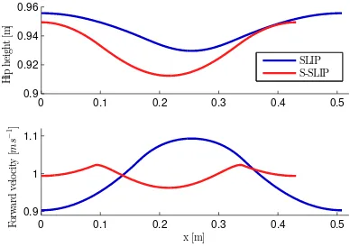
In this work we propose a control strategy for the Seg-mented Spring-Loaded Inverted Pendulum (S-SLIP) model, which is different from the SLIP model in that it has segmented legs with torsional stiffness knees, which is more realistic when compared with existing robot designs, which use knees and leg retraction to avoid food scuffing. For the S-SLIP model, the foot-hip stiffness is nonlinear, arising from the two-link leg geometry. It has been shown that given proper initial conditions, the uncontrolled S-SLIP model exhibits autonomous stable limit cycle running gait [5]. However, the model also shows passive limit cycle walking gait similar to the SLIP model. Fig. 1 shows an S-SLIP walking gait, compared to a SLIP walking gait at an average forward velocity of1.00m s-1. Both systems have equal mass

and leg lengths of _≈ 1.0 m. While the hip trajectories are similar, there is a clear difference in forward velocity profiles.

W. Roozing and R. Carloni are with the Robotics And Mechatronics group, MIRA Institute, University of Twente, The Netherlands. E-mail: [email protected], [email protected]

0 0.1 0.2 0.3 0.4 0.5

0.9 0.92 0.94 0.96

H

ip

he

ig

ht

[m

]

SLIP S-SLIP

0 0.1 0.2 0.3 0.4 0.5

0.9 1 1.1

x [m]

Fo

rw

ar

d

ve

loc

it

y

[

m

s

−

1]

Fig. 1. SLIP vs S-SLIP walking gaits at average velocities of 1.00 m s-1_{. Both systems have equal mass and leg lengths of≈1.0 m. While the}

trajectories are comparable, there is a difference in forward velocity profile due to high stiffness of the segmented leg just after impact.

The segmented leg has high stiffness just after impact due to its configuration, which quickly decreases as the leg is compressed. The result is that the forward velocity is reduced during double support when compared to the linear leg of the SLIP model.

The control strategy developed in this work uses variable leg stiffness to stabilise the system after a disturbance and from one limit cycle walking gait to another. The perfor-mance of this strategy is shown by a simulated controlled S-SLIP system that switches between two gaits with a large forward velocity difference.

Furthermore, a realistic bipedal robot model is designed that uses Variable Stiffness Actuators (VSAs) to control the knees and thus leg stiffness. The control is based on the developed strategy for the S-SLIP model, and is extended with additional components to facilitate leg swing and leg retraction, which arise due to the additional dynamics of this model. A reference gait is obtained by using this model with constant leg stiffness. The variable leg stiffness is then used to stabilise the system into this gait and to inject energy losses generated by foot impacts. It is shown that this results in a stable limit cycle walking gait.

y

x m

ζ1 ζ2

c2 c1

β2 β1

λ1

λ2

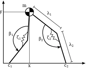
Fig. 2. The S-SLIP model consists of a hip point mass, with two massless segmented legs with links of lengthλ1 andλ2. In the knees with angles

β1 andβ2 there are torsional springs with stiffnessesζ1 andζ2. The legs

touch the ground at the foot contact pointsc1 andc2.

ytd

Lg

VLO VLO

α0

DS

SS SS

β0

L2=L0

L1

Fig. 3. A single step of the S-SLIP model, shown at touch-down. The leg that has just touched down is at its rest lengthL0and rest knee angle

β0, and the virtual leg from hip mass to foot contact (dashed line) is at an

angleα0with the ground. The step starts and ends at VLO and has length

Lg. The virtual leg lengths are defined asL1andL2. At touch-down, the

system transitions to double-support (DS) phase, during which both legs are in contact with the ground. The transition back to single-support (SS) occurs when the trailing virtual legL1reaches its rest length. Touch-down

and lift-off occur when the hip mass crosses the touch-down heightytd.

II. SEGMENTEDSPRING-LOADEDINVERTEDPENDULUM (S-SLIP)

In this Section the S-SLIP model is described. We describe the configuration manifold and conditions for state transition. Next the system dynamics are derived and we conclude with a S-SLIP limit cycle gaits and a normalised description.

A. Configuration Manifold & State Transitions

The Segmented Spring-Loaded Inverted Pendulum (S-SLIP) model is shown in Fig. 2. It consists of a hip point mass m, connected to two massless segmented legs, each composed of two links with upper leg lengthλ1 and lower leg lengthλ2. Between the links there are torsional springs with stiffnesses ζ1 and ζ2, and the knee angles are defined asβ1andβ2. The foot contact points are denoted byc1 and c2.

The configuration of the system is given by the position of the hip mass as (x, y) =: q _{∈ Q}, and its velocity by

˙

q _∈ Tq_Q, the tangent space to _Q at q. The system state is then given as x := (q,p), with the momentum p := (px, py) =Mq˙ and the mass matrix M = diag(m, m).

As in [4] and [6], a single step is defined as a trajectory q(t) _{∈ Q} that starts with the system in Vertical Leg Orientation (VLO), where the hip mass is exactly above the supporting leg. The step ends when the system again reaches VLO (Fig. 3), and the role of the legs is then exchanged. We define the gait lengthLg :=x(T), where T is the gait time period, i.e.q(t) =q(t+T)after which a new step starts.

Every step consists of two distinct phases, i.e. single-support (SS) and double-single-support (DS) during which either one or two legs are in contact with the ground, respectively. The SS→DS transition occurs when the swing leg touches down, when the length is equal to the rest lengthL0, that is, the length of the leg when the knee is at its rest angleβ0:

L0=

q λ2

1+λ22−2λ1λ2cos (β0) (1) At this moment the hip mass is at the touch-down heightytd, corresponding to the angle-of-attackα0, i.e. at touch-down the leading leg is at an angle α0 with the ground so that y = ytd := L0sin(α0). At this moment, the foot contact

point isc2=x+L0cos(α0).

Conversely, the DS→SS transition occurs when the trailing leg reaches its rest length. The swing leg disappears, and reappears at the subsequent moment of touch-down, which is possible because the leg is massless. In the nominal case, only the trailing leg reaches its rest length and contactc2 is relabeled asc1to correspond to the notation used during SS phase. During SS, the swing leg knee is at its rest angle, i.e. β2_≡β0 and the leg exerts no force. We can now define two subsets of _Q which correspond to the single- and double-support phases respectively:

QSS={q∈ Q |y > ytd, y < L0}

QDS={q∈ Q |y < ytd, y >0}

(2)

where the conditionsy < L0 andy >0 assure to avoid the

remaining cases, i.e. lift-off and fall respectively. Note that for a walking gaitq∈ QSS∪ QDS.

During contact, the lengthLi of each leg is given by

Li =

q

(x₋ci)2+y2_{, i∈ {1,2} (3)}

with corresponding knee angleβi

βi= cos−1

λ21+λ22−L2i

2λ1λ2

, i∈ {1,2} (4)

Remark:Lift-off is also possible whileq∈ QSS∪ QDS. We take care of this in simulation by checkingL1≤L0∨L2≤

L0, i.e. at least one leg is in contact with the ground.

B. System Dynamics

To derive the dynamic equations for the system, we use the Hamiltonian approach. The kinetic energy function is defined asK= 1

2p

T_M−1_{pand the potential energy function as}

V =mgy+1

2ζ1(β0−β1)

2

+1

2ζ2(β0−β2)

α0

ζ0

xavg Natural gaits

for fixed (α0, ζ0, β0)

Values of (α0, ζ0, β0) for

which natural gaits exist β0=150°

β0=170°

β0=...

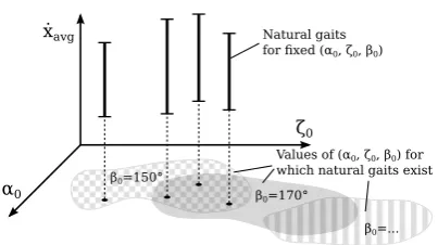
Fig. 4. Average forward velocities x˙avg of natural gaits for different values of(α0, ζ0, β0). Note that for given(α0, ζ0, β0), the average forward

velocity is proportional to the system energyH.

wheregis the gravitational acceleration. The dynamic equa-tions are then defined by the Hamiltonian energy function

H =K+V as

d dt q p = 0 I

−I 0

"δH δq δH δp # (5)

Note that a solutionq(t)of (5) is of classC2_{, due to the} non-differentiability of the leg forces at the moment of transition between the single- and double-support phases.

C. S-SLIP Limit Cycle Gaits

A limit cycle gait is a periodic walking gait, which returns to the same state periodically. From this point on, we refer to limit cycle walking gaits of the S-SLIP model asnatural gaits.

In the description of natural gaits, we use the state at VLO as initial conditions, i.e.x0= (q,p)0= (x, y, px, py)0, and, during walking in natural gait, the system returns to this state at every VLO. Since we can take at every VLO x_≡ 0, a

natural gait can then be fully described as

Σ = (α0, ζ0, L0, m, β0, y0, px,0, py,0) (6)

where ζ0 is the nominal knee stiffness and ζ1 =ζ2 =ζ0. Note that it is not possible to use the total system energyH to uniquely describe a natural gait, because energy can be stored in either potential (leg compression, hip height) or kinetic (hip momentum) energy. As natural gaits exist for ranges of parameters, there often exists a range of natural gaits that achieve a desired forward velocity (Fig. 4). Conversely, a single set (α0, ζ0, β0) can often achieve a range of average forward velocities (vertical bar in Fig. 4).

D. Normalised Notation of S-SLIP Limit Cycle Gaits

The torsional knee stiffness ζ0 and energy H can be normalised in dimensionless form as

˜

ζ= ζ0

mgL0 H˜ =

H

mgL0 (7)

If we normalisexas x˜:= (˜q,p˜) = (˜x,y,˜ px,˜ py˜ )with

˜

x= x

L0 y˜=

y

L0 px˜ =

px

m√L0g py˜ =

py

m√L0g (8)

and use (7), we obtain a fully normalised unique descrip-tion_Σ˜ _{of a natural gait:}

˜

Σ =α0,ζ, β0,˜ y0,˜ px,0,˜ py,0˜ (9)

The gait trajectory can then be found by solving (5) for

˜

Σ. Using this description, equal gaits on different S-SLIP

systems now result in the same normalised state trajectory

˜

x(t) = (˜q(t),p˜(t)). Similarly to px,˜ py˜ , the velocities are

normalised as

˙˜

x= √x˙

L0g y˙˜=

˙

y

√

L0g (10)

Note that the normalisation x˙˜ is the Froude number F r [9], [10], used to compare the relative walking speeds of systems with different leg lengths.

III. S-SLIP CONTROL DESIGN

The control design of the controlled S-SLIP model is inspired by [6]. By actively controlling the leg stiffness of the legs, the rejection of external disturbances to the system can be significantly increased. Furthermore, after a disturbance, the system can be stabilised into its original gait by injecting or removing energy appropriately.

The knee stiffnesses are defined asζi =ζ0+ui, i∈ {1,2}

(Fig. 2) with the control inputs ui restricted to subsets Ui = {ui ∈ R|0 < ζ0+ui < ∞}, such that the result is a meaningful stiffness value. We intend to control the system towards a reference gait _Σ˜ _{with normalised state}

trajectoryx˜(t), i.e. to a reference state trajectoryx˜o_(t)such that ui _→ 0, i _{∈ {}1,2_}. However, during single-support phase the system has only one control input and x˜o_(t) cannot be tracked exactly, which may lead to instability as the system lags behind the reference. As ˜x was identified to be a periodic variable and required to be monotonically increasing in time, the references are reparametrised on x˜.

The references y˜∗(˜x),x˙˜∗(˜x) are then sufficiently described

as

˜

y∗(˜x) = ˜yo_{(˜x) x˙˜}∗_{(˜x) = ˙˜x}o_{(˜x) (11)}

However, as a general analytic expression for the spring-loaded pendulum does not exist [11], a Fourier series expan-sion approximation of the numerical solution is used. We extend Eq. (5) to obtain

d dt q p = 0 I

−I 0

"δH δq δH δp # + 0 B u (12)

withu= [u1, u2]the controlled part of the leg stiffness. The

input matrixB is given by

B=

"dφ1

dx dφ2 dx dφ1 dy dφ2 dy # (13) with

φi= 1

2(β0−βi)

2

calculated from (3)–(4). To formulate the control strategy, we rewrite Eq. (12) in standard form as

˙

x=f(x) +X

i

gi(x)ui (15)

and then define error functions h1 andh2 as h1=y−y∗

h2= ˙x₋x˙∗ (16)

The control solution is then given as follows. • Forq∈ QSS and|x−c1| ≤:

u1= 1

Lg1Lfh1

−L2fh1−κdLfh1−κph1

u2≡0

(17)

• Forq∈ QSS and|x−c1|> :

u1= 1

Lg1h2

(₋Lfh2₋κvh2)

u2≡0

(18)

• Forq∈ QDS:

u1 u2

=A−1

−L2

fh1−κdLfh1−κph1

−Lfh2−κvh2

(19)

with

A=

Lg1Lfh1 Lg2Lfh1

Lg1Lfh2 Lg2Lfh2

(20)

whereL2

fhi,Lfhi,LgihiandLgiLfhidenote the (repeated) Lie-derivatives ofhi along the vector fields defined in (15), κd, κp, κv are tunable control parameters and ∈ [0,1₂Lg]

is the distance around VLO during which h1 should be controlled instead of h2. The control inputs (17), (18), (19) ensure that the errorh1converges asymptotically to zero and that the errorh2 is at least bounded [6].

Remark: Due to only one control input being available during single-support phase, the system is not always fully controllable. Because at VLO the velocity error cannot be controlled due to leg orientation, we choose to control the hip height error h1 around VLO and control the velocity errorh2 just after touch-down and just before lift-off.

A. Gait Switching

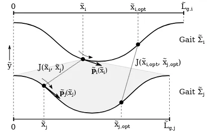
1) Finding Optimal Points: Suppose that two natural gaits

˜

Σi and Σ˜j, with step lengths Lg,i,˜ Lg,j˜ respectively, have been chosen and that we want the system to switch from_Σ˜_i

to_Σ˜_{j. The parametrisation of both can be used to determine}

exactly how to transition from one gait to the other. In each gait one point should be considered: The point in_Σ˜_{iat which}

the switch is executed and the point in_Σ˜_{jto switch into. Any}

point˜xi_∈h0,Lg,i˜ on one step of_Σ˜_{ican be associated with}

any pointxj˜ _∈h0,Lg,j˜ on one step of _Σ˜_{j. To find this set}

of points(˜xi,opt,xj,opt˜ ), we minimise the criterionJ(˜xi,xj˜ )

w.r.t. (˜xi,˜xj):

J(˜xi,xj˜ ) =µ1|yj˜ (˜xj)−yi˜(˜xi)|+

µ2xj˙˜ (˜xj)₋xi˙˜(˜xi)+

µ3yj˙˜(˜xj)₋yi˙˜(˜xi)

(21)

0

0 y ~

J(x~i, x~j) xi

~ _x

i,opt ~

J(x~i,opt, x~j,opt) Gait Σi

~ Lg,i ~

pj(xj)

~ ~

pi(xi)

~ ~ xj ~ _x j,opt ~ Lg,j ~

Gait Σj ~

Fig. 5. Optimisation of the switching point from_Σ˜_itoΣ˜_{j. The pointx˜iis} moved along one step of_Σ˜_{i, andJ(˜xi,˜xj)is then calculated for all values} of˜xjin one step ofΣ˜j. Minimisation ofJfor both these parameters then results in the optimal switching points(˜xi,opt,˜xj,opt).

By choosing the weights {µ1, µ2, µ3_}, the different aspects of the gait can be emphasised as to achieve a smooth response. Note that multiple minima may exist, so we search for the global minimum. Due to the use of normalised variables the results are again identical for the same natural gaits on different SLIP systems, and due to symmetry results obtained for _Σ˜_{i → Σ}˜_{j are also valid for Σ}˜_{j →Σ}˜_{i. In the}

next sections we outline the switching strategy. Although the method is general, we make a distinction between switching between gaits with equal values of (α0,ζ˜) and gaits with

different(α0,ζ˜). The first case will be shown to be a special

case of the second.

2) Instantaneous Switching: In the case in which(α0,ζ˜)

remain constant, we can switch the references of the S-SLIP controller instantaneously at the desired point, and we need only to redefine the controller references y˜∗(˜x),x˙˜∗(˜x)as:

˜

y∗(˜x) =

˜

yi(˜x) x <˜ S˜opti,j

˜

yj(˜x₋xδ,j˜ ) x˜_≥S˜opti,j

˙˜

x∗(˜x) =

_˙˜

xi(˜x) x <˜ S˜opti,j

˙˜

xj(˜x₋xδ,j˜ ) x˜_≥S˜opti,j

(22)

where _S˜i,j

opt is the normalised switching distance which coincides with the pointxi˜ on the current gait. The reference of _Σ˜_{j is shifted by xδ,j˜ such that the points (˜xi,opt,xj,opt˜ )}

align at_S˜i,j

opt.

3) Gait Interpolation: In the case the two gaits have different values of(α0,ζ˜), we ensure the value ofα0is con-tinuous inx˜. We extend (22) with a transition period, during

the corresponding values ofα0 andζ˜:

˜

y∗(˜x) =

  

˜

yi(˜x) β_≤0

(1₋β)˜yi(˜x) +βyj˜ (˜x₋xδ,j˜ ) 0< β <1 ˜

yj(˜x−xδ,j˜ ) β≥1

˙˜

x∗(˜x) =

  

˙˜

xi(˜x) β_≤0

(1₋β) ˙˜xi(˜x) +βxj˙˜ (˜x₋xδ,j˜ ) 0< β <1 ˙˜

xj(˜x) β_≥1

α0=

  

α0,i β_≤0

(1₋β)α0,i+βα0,j 0< β <1

α0,j β_≥1

˜ ζ=    ˜

ζi β_≤0

(1₋β)˜ζi+βζj˜ 0< β <1

˜

ζj β≥1

(23) where the interpolation factor β is defined as β = (˜x₋

˜

Sopti,j)/γ. The parameter γ ≥ 0 is the transition length. By the definition of the normalised variables, γ effectively is the number of leg lengths inxto interpolate for. Of course,

˜

y∗_,x˙˜∗_{in (23) converge to (22) as γ→0. The reason we} use (22) for constant(α0,ζ˜)is that then we let the controller handle the transition as quickly as it can, instead of forcing a transition period of fixed length.

IV. S-SLIP SIMULATION RESULTS

To demonstrate the effectiveness of the method for forward velocity differences, a slow gait with an average velocity of 0.259 (0.811 m s-1_{) and (α0,ζ}˜_{) = (70,0.224) and a fast}

gait with an average velocity of 0.457 (1.429 m s-1_{) and} (α0,ζ˜) = (65,0.224) are chosen, to demonstrate robustness

against changing the angle of attack. Here we use the gait interpolation withγ= 1.0(Sec. III-A.3). Furthermore,m= 80 kg,λ1 =λ2 = 0.50m, β0 = 170 deg (s.t.L0 ≈0.996

m), {µ1, µ2, µ3} = {15,2,5} and for the S-SLIP control

{, κp, κd, κv}={0.1,50,25,50}. From _ζ˜_{= 0.224 follows}

ζ0≈175N m rad-1(Eq. (7)). Simulations were performed in

Mathworks MATLAB R2012b, using the ode45 solver with absolute and relative tolerances of 1e-11. The velocity ranges were found by fixing the vertical velocity at VLO to zero, thus enforcing symmetrical gaits [4], and incrementing the forward velocity at VLO in small steps. The system starts in the slow gait (gait 1), is commanded to change to fast gait (gait 2) at 1.0 m, and then to switch back to the slow gait (gait 3 = gait 1) at 5.5 m.

Fig. 6 shows the resulting hip trajectory with the de-sired and optimal switching points indicated. The trajectory smoothly lowers to the new hip height as its shape transforms into that of the second gait. Fig. 7 shows the hip height and forward velocity over time, which converge to the new gait in approximately 5 steps. Fig. 8 shows the corresponding control input and error functions. On a few occasions, the stiffness of the trailing leg reaches the lower limit due to the system attempting to slow down. After transition, the leg stiffnesses converge to the nominal ζ0 value. Note that during single-support, the stiffness of the swing leg is always equal toζ0, asu2˜ ≡0 in that case (Eq. (17)–(18)).

0 1 2 3 4 5 6 7 8

0.88 0.9 0.92 0.94 0.96 ˜ x ˜ y System

Switch gait 1→2

Switch gait 2→3

Fig. 6. Hip trajectory for the transition from slow to fast gait and back for two gaits with different(α0,ζ˜). For each pair of vertical dashed lines, the

first indicates the commanded switching distance, and the second indicates the resulting optimal switching distance.

0 1 2 3 4 5 6 7

0.88 0.9 0.92 0.94 0.96 0.98 time [s] ˜ y

0 1 2 3 4 5 6 7

0.2 0.3 0.4 0.5

time [s]

˙ ˜x

System Gait 1 reference Gait 2 reference Gait 3 reference

Fig. 7. Hip height and forward velocity over time. The system converges to the new gait in approximately 5 steps.

Fig. 9 shows the energy balance. Most of the total energy increase on transition is put into (forward) kinetic energy, to accommodate the faster gait.

V. BIPEDAL ROBOT MODEL

The bipedal robot model is based on the mechanical design of an existing bipedal walker [7] (Fig. 10). It is a four-link model with segments of length λ1 and λ2 similar to the S-SLIP model. However, the hip mass is replaced by two separate upper-leg massesmh,l, mh,r – there is a small mass difference between left and right on the physical robot due to electronics and a guide rail – and two lower-leg masses ml are added (Fig. 11). The hip joint position is denoted

0 1 2 3 4 5 6 7 0 200 400 600 time [s] ζ0 + u1 , ζ0 +

u2 ζ0+

u₁ ζ0+u₂ ζ0

0 1 2 3 4 5 6 7

−0.02 −0.01 0 0.01 0.02 time [s] P o si ti o n er ro r

0 1 2 3 4 5 6 7 −0.4

−0.2 0 0.2 0.4 V el o ci ty er ro r Position error Velocity error

Fig. 8. Control input and error functions. The leg stiffness converges to a constant value after rejection of the transition disturbances. Note that during single-support, the stiffness of the swing leg is always equal toζ0,

asu˜2≡0in that case (Eq. (17)–(18)).

0 1 2 3 4 5 6 7

−0.2 0 0.2 0.4 0.6 0.8 1 1.2 time [s] N o rm a li se d en er g y Kinetic energy Potential energy Elastic energy Control potential energy Total energy

Fig. 9. Energy balance. The total energy increases on transition to the second gait, mostly reflected in kinetic energy resulting from the increased forward velocity.

generated by simplified Variable Stiffness Actuator (VSA) models (Sec. V-A). The foot contact points are denotedcl, cr, similar to the S-SLIP model. The ground contact forces are modeled using the Hunt-Crossley contact model. The robot is constrained to the sagittal plane using constraint forces.

A. Variable Stiffness Actuator (VSA)

Variable Stiffness Actuators (VSAs) belong to a class of actuators which are able to change their apparent output stiff-nessKindependently of their output equilibrium position by proper control of their internal degrees of freedom z (Fig. 12).

The used design is based on the principle of a lever arm with length d, with a movable pivot of which the position is given by z1 ∈ [0, d] (Fig. 13), which changes

the transformation ratio between change in output position and change in spring state. For the analysis we use the port-Hamiltonian method, using a Dirac structure. For more details, see [12]. For Fig. 13, the spring state s(z) with z= [z1, z2]is given as

s= d

q1(d−z1) sin(r−z2) (24)

Fig. 10. The bipedal robot model is based on the mechanical design of a bipedal walker in our lab, with realistic body dynamics, friction and ground contact forces. y x mh,r ηr ηl βl λ1 λ2 mh,l ml ml τl τr τh αr αl θ βr

Fig. 11. Bipedal robot model. The model is similar to the S-SLIP model, with the hip mass replaced by two upper-leg masses and the addition of two lower-leg masses.

in which small deflections are considered, i.e.r−q2≈0:

s_≈ d

z1(d−z1)(r−z2) (25)

The apparent output stiffness K of the actuator is then given by

K=kd

z1(d−z1) (26)

where k is the stiffness of the internal spring. It is clear that for z1 =d, K _≡0 and for z1 = 0, K _{≡ ∞}. Eq. (26) is not a function of z2, such that the equilibrium position

z2 K(z₁) r

Fig. 12. Variable stiffness actuator with internal degrees of freedomz= [z1, z2]. The stiffnessKat the output linkris controlled independently of

the equilibrium positionz2 by the stiffness controlling variablez1.

d

z1

s r

Fig. 13. Output stiffness changing mechanism based on the principle of changing the transformation ratio between an internal spring and the output link. A lever with lengthdwith movable pivotz1 connects the outputr