ISSN Online: 2162-2086 ISSN Print: 2162-2078
DOI: 10.4236/tel.2018.81007 Jan. 29, 2018 111 Theoretical Economics Letters
Value-at-Risk Based on Time-Varying Risk
Tolerance Level
*
Debasish Majumder
Reserve Bank of India, Kolkata, India
Abstract
The conventional judgement-based method for fixing the risk tolerance level in the Value-at-Risk (VaR) model might be a suboptimal method, because the procedure induces the possibility of bias in risk measurement. Conversely, a superior risk management practice might be one, where input parameters are determined by a quantitative process which is “non-subjective to the risk modeller’s preferences”. Based on this insight, we have improved on the VaR model. Our model allows time variation of the risk tolerance level and so is suitable for scenario-wise risk analysis.
Keywords
Value-at-Risk, Extreme Value Theory, Generalised Pareto Distribution, Tail-Related Risk Models
1. Introduction
A class of risk measures, which are commonly referred to as “tail-related risk measures” in the economic literature, is based on basics of fixing ex-ante a risk tolerance level. Value-at-Risk is a common example of this class. Risk tolerance is the level of risk that an investor is willing to take. But, gauging risk appetite accurately can be a tricky task. In practice, the risk tolerance level is generally decided by judgement/or perception by a risk manager or a risk management committee or, in certain cases, an external regulatory body. For this purpose, it has been a common practice to follow recommendations by the BASEL commit-tee of banking supervision. At present, BASEL guidelines are 99% and 99.9% confidence level for Value-at-Risk (VaR) and 97.5% confidence level for Ex-pected Shortfall (ES) [1]. Most probably, those recommendations are drawn on the basis of country-wise experiences of analysing large set of historical data. Al-*The views expressed in this paper are of the author and not of the organization to which he belongs. How to cite this paper: Majumder, D. (2018)
Value-at-Risk Based on Time-Varying Risk Tolerance Level. Theoretical Economics Let-ters, 8, 111-118.
https://doi.org/10.4236/tel.2018.81007
Received: November 15, 2017 Accepted: January 26, 2018 Published: January 29, 2018
Copyright © 2018 by author and Scientific Research Publishing Inc. This work is licensed under the Creative Commons Attribution International License (CC BY 4.0).
DOI: 10.4236/tel.2018.81007 112 Theoretical Economics Letters ternatively, in certain cases, the risk modeller adopts commonly used percent-ages viz. 99%, 95% and 90% for this purpose. Majumder [1], however, docu-mented evidence from various developed and emerging equity markets of those incidents where a minor change in the risk tolerance level translated into a large difference in VaR. Nevertheless, such instances are not uncommon in financial markets. Similar observations were documented by Degennaro [2] who formed examples to establish that non-cooperative choices of the risk tolerance level by two investors were resulting in a substantial variation in their VaR estimates. Therefore, in many occasions, the risk modeller’s preferences on the risk toler-ance level could have large impacts on the tail measure. When those preferences are biased,being over concerned to the high volatile period/or stress or due to any other reason, the bias would be transfused into the tail measure. In this ap-proach, the risk tolerance level, which was decided ex-ante during turbulence, maybe appropriate for the turbulent period. However, the same could be subop-timal for quiet periods. Logically, it is extremely difficult to get a risk tolerance level which is suited uniformly across scenarios and this is perhaps a reason for model risk in the conventional approach.
In an alternative approach, the present paper proposes that the risk tolerance level ought not to be pre-assigned, but may be determined by the model itself. In this framework, this parameter may vary with the shape of the loss distribution. One way to determine the same might be using the Pickands-Balkema-de Haan theorem which essentially says that, for a wide class of distributions, losses which exceed the high enough threshold follow the generalized Pareto distribu-tion (GPD) [3] [4]. Using this theorem, it is easy to establish that the extreme right tail part of a distribution asymptotically converges to the tail of a general-ised Pareto distribution (GPD). This hypothesis reveals that we can always find a region in the extreme right tail of the loss distribution, for which the equivalent region from a suitable GPD is available. Therefore, there exists a threshold, data above which shows generalized Pareto behavior. The threshold would essentially be reasonably large to cover all events which are “extreme” in nature. Naturally, events belonging to the rest of the distribution are “normal” or “non-extreme” in nature. The procedure gives us the opportunity to estimate simultaneously the tail size and the starting point of the tail. In other words, it allows simultaneous estimation of VaR and the risk tolerance level. The rest of the paper is organized as follows: Section 2 describes the model. Section 3 provides empirical findings and Section 4 concludes.
2. The Model
2.1. Behaviour of Losses Exceeding a High Threshold
DOI: 10.4236/tel.2018.81007 113 Theoretical Economics Letters [5], the distribution function
( )
FY1u of the truncated loss (Y1u) (truncated at thepoint u) can be defined as:
( )
[
]
( )
( )
( )
1 1
0 if if 1
u u X X
Y
X
x u F x F u
F x P Y x P X x X u x u
F u
≤
−
= ≤ = ≤ > = >
−
Based on FY1u, we can define the distribution function of the excess over a
high threshold u:
( )
[
]
(
)
( )
( )
1
u X X
Y
X
F x u F u
F x P X u x X u
F u
+ − = − ≤ > =
− (1)
for 0≤ <x x u0− .
Balkema and de Haan [3] and Pickands [4] showed that, for a large class of distributions, the generalised Pareto distribution (GPD) is the limiting distribu-tion for the distribudistribu-tion of the excess, as the threshold (u) tends to the right endpoint. According to this theorem, we can find a positive measurable function
( )
uσ such that
( )
( )( )
0 0 0 Yu , u 0
u xLim Sup→ ≤ < −x x u F x G− ξ σ x = (2)
where the distribution function of a two parameter generalised Pareto distribu-tion with the shape parameter (ξ), and scale parameter (σ
( )
u ) has the follow-ing representation:( )
(
(
( )
)
)
1, ( )
1 1 ( ) if 0 1 exp if 0
u x u G x x u ξ ξ σ
ξ σ ξ
σ ξ − − + ≠ = − − =
where σ >0, x≥0 when ξ ≥0 and 0≤ ≤ −x σξ when ξ <0. (2) holds if
and only if F belongs to the maximum domain of attraction of the generalised extreme value (GEV) distribution (H) [6]. The equivalent representation of (2) could be in terms three parameter GPD: forx u− ≥0, the distribution function
of the three parameter GPD
(
Gξ, , uσ( )
x)
can be expressed as the limiting dis-tribution function of the excess. Gξ, , u σ( )
x with shape parameter (ξ), location parameter (u) and scale parameter (σ) has the following representation.( )
(
(
)
)
(
)
(
)
1
, ,
1 1 - if 0 1 exp - if 0
u x u G x x u ξ ξ σ
ξ σ ξ
σ ξ − − + ≠ = − − =
where σ >0,
(
x u−)
≥0 when ξ ≥0 and 0≤(
x u-)
≤ −σξ whenξ <0.This representation would provide us a theoretical ground to claim that there exists a threshold, the data above which would have generalized Pareto be ha-viour.
2.2. Identifying the Tail Region
DOI: 10.4236/tel.2018.81007 114 Theoretical Economics Letters written:
(
)
( )
, ,( )
(
1( )
)
X X u X
F x u+ ≈F u G+ ξ σ x −F u
Setting y = x + u
( )
( )
, ,(
)
(
1( )
)
X X u X
F y ≈F u G+ ξ σ y u− −F u (3)
The right hand side of the Equation (3) can be simplified in the form of a dis-tribution function of a GPD:
( )
,(
)
X
F y ≈Gξ σ y−µ (4)
where σ σ =
(
1−F uX( )
)
ξ and u(
(
1 F uX( )
)
1)
ξ
µ= −σ − − − ξ.
Hence, if we can fit the GPD to the conditional distribution of the excess above a high threshold, it can also be fitted to the tail of the original distribution above a certain threshold [7].
When u is fixed at uˆ, yˆ would be the minimum value of y for which the Equation (4) will hold. The deviation of F yX
( )
from Gξ σ,(
y−µ)
would, therefore, be non-zero for y y< ˆ, which is expected to be zero for all y y≥ ˆ.We may consider an indicator, viz. the cumulative square deviation for y y< 0,
( )
( )
(
)
0
2
0 X ,
y y
D y F y Gξ σ y µ
<
=
∑
− − , which might be useful for identifyingˆ
y. By its nature, D y
( )
0 would be an increasing function of y0 for y0< yˆand would be nearly flat for y0≥ yˆ. Therefore, the slope of the D y
( )
0 wouldbe positive for y0< yˆ, which would be almost zero for y0≥yˆ. We can
iden-tify the cut-off point, yˆ, after which the slope of the D y
( )
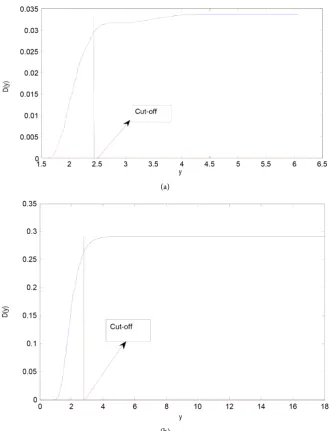
0 would bestatisti-cally insignificant [1]. To test this hypothesis, we have plotted D(y) versus for normal and t distributions (Figure 1). D(y) is almost flat after a certain cut-off in both of these cases which validates our postulate.
Therefore, we can bifurcate the underlying distribution into two parts: X y≥ ˆ
is the risky region of the distribution in the sense that this region could be ap-proximated by the tail of an equivalent GPD. All large unforeseen losses would belong to this part. Conversely, X y< ˆ is the region of the distribution which
does not cause severe tail risk.
2.3. Measuring the Tail Risk
For a small quantile of order p, P= −1 F yX
( )
ˆ < yˆ, we can write( )
(
1 X ˆ)
(
1 , ( )u0(
ˆ ˆ)
)
P≈ −F u −Gς σ y u− (5)
VaR represents in probabilistic terms a quantile of the loss distribution func-tion FX [8]. Therefore,
ˆ
p
VaR =yVaRp =yˆ (6)
DOI: 10.4236/tel.2018.81007 115 Theoretical Economics Letters (a)
[image:5.595.207.538.69.501.2](b)
Figure 1. Plot of D(y) versus y for normal and t distribution. (a) Plot of D(y) based on Normal Distribution (mean: 0, standard deviation: 1.76); (b) Plot of D(y) based on t dis-tribution (Degrees of freedom: 2.18).
2.4. Simulation Study for Threshold Choice
When the form of the underlying loss distribution FX(.) is known, we can de-velop a procedure for estimating the threshold, u, by a simulation study. We may recall our result in the preceding section that we can get a sufficiently high threshold u, above which the distribution function of the excesses F xYu
( )
canbe approximated by the distribution function of a generalised Pareto distribu-tion, Gξ σ, ( )u
( )
x . Initially, we fix u to some u/ and generate 100 samples each of size 4000 from the underlying distribution FX. If u/ is the true threshold, then the deviation of Gξ σ,( )
u/( )
x from Gξ σ,( )
u/( )
x is expected to be zero for all x u≥ /cu-DOI: 10.4236/tel.2018.81007 116 Theoretical Economics Letters mulative square deviation for x u≥ /,
( )
( )
( )
( )
/ /
2
,
2 u u
Y x u
D u F x Gξ σ x
′ ≥
′ = −
∑
,which might be useful for identifying the threshold. If u/ is the true threshold,
( )
2
D u′ would be zero for each sample. Based on this indicator, we can form a
Mean Squared Error (MSE):
( )
100{
( )
/}
/
1 2 1
100i i
D u MSE u
n =
=
∑
where ni is the number of observation in the ith sample exceeding u/.
( )
MSE u can be computed for various values of u starting from 0. The best es-timate of u (say u) would be one, for which MSE u
( )
is minimum.3. Empirical Findings
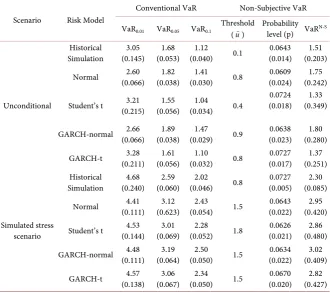
VaR and VaRN-S based on daily returns on S & P 500 Composite Index for the period of 30 years, from 18th February, 1985 to 17th February, 2015, computed using five risk models separately for the full sample and the simulated stress scenario are reported in Table 1. The stress scenario is simulated in the line of Studer [10] and Breuer and Krenn [11], who employed the Mahalanobis distance as a mathematical tool to choose stress scenarios [1]. Additionally, the condi-tional EVT framework proposed by McNeil and Frey [6] was adopted to com-pute VaRN-S for GARCH. For each risk model, in the normal as well as the tur-bulent period, the equilibrium probability level1 in VaRN-S lies in-between 0.05 and 0.1 and the estimate of VaRN-S in-between VaR
0.1 and VaR0.05. Furthermore, similar to the conventional model, the estimate of VaRN-S in the stress scenario is greater than the estimate of the same for the full sample indicating that the new risk measure correctly captures riskiness of markets. Hence, estimates of VaRN-S are not too arbitrary numbers to be accepted the same as a risk measure. Inter-estingly, the standard error of the probability level is low (highest value: 0.024 (Normal (unconditional)). This indicates that additional volatility in VaR due to introduction of time variation in the probability level would be limited.
4. Conclusion
DOI: 10.4236/tel.2018.81007 117 Theoretical Economics Letters
Table 1. A comparison between VaR and VaRN-S based on S & P 500 Composite Index.
Scenario Risk Model
Conventional VaR Non-Subjective VaR
VaR0.01 VaR0.05 VaR0.1 Threshold (u) Probability level (p) VaRN-S
Unconditional
Historical
Simulation (0.145) 3.05 (0.053) 1.68 (0.040) 1.12 0.1 (0.014) 0.0643 (0.203) 1.51 Normal (0.066) 2.60 (0.038) 1.82 (0.030) 1.41 0.8 (0.024) 0.0609 (0.242) 1.75
Student’s t (0.215) 3.21 (0.056) 1.55 (0.034) 1.04 0.4 (0.018) 0.0724 (0.349) 1.33
GARCH-normal (0.066) 2.66 (0.038) 1.89 (0.029) 1.47 0.9 (0.023) 0.0638 (0.280) 1.80
GARCH-t (0.211) 3.28 (0.056) 1.61 (0.032) 1.10 0.8 (0.017) 0.0727 (0.251) 1.37
Simulated stress scenario
Historical
Simulation (0.240) 4.68 (0.060) 2.59 (0.046) 2.02 0.8 (0.005) 0.0727 (0.085) 2.30 Normal (0.111) 4.41 (0.623) 3.12 (0.054) 2.43 1.5 (0.022) 0.0643 (0.420) 2.95
Student’s t (0.144) 4.53 (0.069) 3.01 (0.052) 2.28 1.8 (0.021) 0.0626 (0.480) 2.86
GARCH-normal (0.111) 4.48 (0.064) 3.19 (0.050) 2.50 1.5 (0.022) 0.0634 (0.409) 3.02
GARCH-t (0.138) 4.57 (0.067) 3.06 (0.050) 2.34 1.5 (0.020) 0.0670 (0.427) 2.82
Note: VaR and VaRN-S are average based on 50 estimates. The standard error of the estimate is provided in
the parenthesis. Data Source: Data Stream.
level. Our empirical study based on S & P 500 composite index reveals that the tail risk of the loss distribution is well captured by the new risk measure in the normal as well as in the stress scenarios. The significance of the research is two-fold: a) reduction of bias by minimising the scope of human intervention in risk measurement which is of practical as well as of social significance and b) gauging risk appetite methodically which is of academic significance. The approach may widen the applicability of tail-related risk models in institutional and regulatory policymaking. At this stage, however, it is not possible to provide the method for backtesting the new VaR model. This might be the topic for future research.
Acknowledgements
The author is grateful to Prof. Romar Correa, former Professor of Economics, University of Mumbai and Prof. Raghuram Rajan, Katherine Dusar Miller Dis-tinguished Professor of Finance at University of Chicago Booth School of Busi-ness and former Governor of Reserve Bank of India for their insightful com-ments/suggestions. He is also thankful to Chief Science Officer, Dr. Chitro Ma-jumdar, RsRL (R-square Risk Lab) for his contribution and inspiration at the in-itial stage of this study.
References
DOI: 10.4236/tel.2018.81007 118 Theoretical Economics Letters Value-at-Risk—Is It a Better Alternative to BASEL’s Rule Based Strategy? Journal of Contemporary Management, 5, 71-85.
[2] Degennaro, R.P. (2008) Value-at-Risk: How Much Can I Lose by This Time Next Year? The Journal of Wealth Management, 11, 92-96.
https://doi.org/10.3905/JWM.2008.11.3.092
[3] Balkema, A.A. and de Haan, L. (1974) Residual Lifetime at Great Age. Annals of Probability, 2, 792-804. https://doi.org/10.1214/aop/1176996548
[4] Pickands, J. (1975) Statistical Inference Using Extreme Order Statistics. Annals of Statistics, 3, 119-131. https://doi.org/10.1214/aos/1176343003
[5] Hogg, R.V. and Klugman, S.A. (1984) Loss Distributions. Wiley, New York. https://doi.org/10.1002/9780470316634
[6] McNeil, A.J. and Frey, R. (2000) Estimation of Tail-Related Risk Measures for Het-eroscedastic Financial Time Series: An Extreme Value Approach. Journal of Em-pirical Finance, 7, 271-300. https://doi.org/10.1016/S0927-5398(00)00012-8 [7] Reiss, R-D. and Thomas, M. (1997) Statistical Analysis of Extreme Values.
Birk-häuser, Basel. https://doi.org/10.1007/978-3-0348-6336-0
[8] McNeil, A.J., Frey, R. and Embrechts, P. (2005) Quantitative Risk Management. Princeton University Press, Princeton, NJ.
[9] Yadav, V. (2008) Risk in International Finance. Routledge, Abingdon.
[10] Studer, G. (1999) Market Risk Computation for Nonlinear Portfolios. Journal of Risk, 1, 33-53. https://doi.org/10.21314/JOR.1999.016
[11] Breuer, T. and Krenn, G. (1999) Stress Testing. Guidelines on Market Risk. Oesterreichische National Bank, Vienna.