ISSN Online: 2161-7198 ISSN Print: 2161-718X
DOI: 10.4236/ojs.2018.81005 Feb. 2, 2018 49 Open Journal of Statistics
The Method of Finite Difference Regression
Arjun Banerjee
Computer Science Department, Purdue University, West Lafayette, IN, USA
Abstract
In this paper1 I present a novel polynomial regression method called Finite
Difference Regression for a uniformly sampled sequence of noisy data points that determines the order of the best fitting polynomial and provides esti-mates of its coefficients. Unlike classical least-squares polynomial regression methods in the case where the order of the best fitting polynomial is unknown and must be determined from the R2 value of the fit, I show how the t-test
from statistics can be combined with the method of finite differences to yield a more sensitive and objective measure of the order of the best fitting poly-nomial. Furthermore, it is shown how these finite differences used in the de-termination of the order, can be reemployed to produce excellent estimates of the coefficients of the best fitting polynomial. I show that not only are these coefficients unbiased and consistent, but also that the asymptotic properties of the fit get better with increasing degrees of the fitting polynomial.
Keywords
Polynomial Regression, t-Test, Finite Differences
1. Introduction
In this paper I present a novel polynomial regression method for a uniformly sampled sequence of noisy data points that I call the method of Finite Difference Regression. I show how the statistical t-test2 can be combined with the method
of finite differences to provide a more sensitive and objective measure of the or-der of the best fitting polynomial and produce unbiased and consistent estimates of its coefficients.
1Portions of this independent research were submitted to the 2013 Siemens Math, Science, and
Technology Competition, and to the 2014 Intel Science Talent Search Competition for scholarship purposes. It received the Scientific Research Report Badge from the latter competition.
2The t-test often called Student’s t-test was introduced in statistics by William S. Gosset in 1908 and
published under the author’s pseudonym “Student” (see [10]). How to cite this paper: Banerjee, A. (2018)
The Method of Finite Difference Regres-sion. Open Journal of Statistics, 8, 49-68.
https://doi.org/10.4236/ojs.2018.81005
Received: December 23, 2017 Accepted: January 30, 2018 Published: February 2, 2018
Copyright © 2018 by author and Scientific Research Publishing Inc. This work is licensed under the Creative Commons Attribution International License (CC BY 4.0).
http://creativecommons.org/licenses/by/4.0/
DOI: 10.4236/ojs.2018.81005 50 Open Journal of Statistics Regression methods, also known as fitting models to data, have had a long history. Starting from Gauss (see [1] pp. 249-273) who used it to fit astronomical data, it is one of the most useful techniques in the arsenal of science and tech-nology. While historically it has been used in the “hard” sciences, both natural and biological, and in engineering, it is finding increasing use in all human en-deavors, even in the “soft” sciences like social sciences (see for example [2]), where data is analyzed in order to find an underlying model that may explain or describe it.
Polynomial regression methods are methods that determine the best poly-nomial that describes a sequence of noisy data samples. In classical polypoly-nomial regression methods when the order of the underlying model is known, the coef-ficients of the terms are estimated by minimizing the sum of squares of the resi-dual errors to the fit. For example, in classical linear regression (see [2] pp. 675-730) one assumes that the order of the fitting polynomial is 1 and then proceeds to find the coefficients of the best fitting line as those that minimize the sum of the squares of its deviations from the noisy samples. The same method can be extended to polynomial regression. On the other hand, when the model order is unknown, the order of the best fitting polynomial must be determined before finding the coefficients of the polynomial terms. In classical regression methods this order is determined from the R2 value of its fit. More on these two
different aspects of polynomial regression are provided below.
1) Determining the order of the best fitting polynomial (Model order un-known)
In classical regression, the goodness of the order of the fitting polynomial is given by the R2 value of the best fitting polynomial—the greater the R2 value the
better the fit. However, this means that one can go on fitting with higher degree polynomials and thereby increasing R2 values. Given the insensitivity of these R2
values (see for example Section 2.4) it is indeed hard to find a stopping criterion. To get around this problem, heuristic methods like AIC, BIC, etc. (see [3] for example) that penalize too many fitting parameters have been proposed. In con-trast, in the method of Finite Difference Regression described below, the order of the best fitting polynomial is determined by using a t-test, namely determining the index of a finite difference row (or column) that has a high probability (beyond a certain significance level) of being zero. The sensitivity of this method is high compared to classical regression methods as I shall demonstrate in Sec-tion 2.5.
2) Determining the coefficients of the best fitting polynomial (Model order known/determined)
DOI: 10.4236/ojs.2018.81005 51 Open Journal of Statistics and consistent, but also that the asymptotic properties of the fit get better with increasing degrees of the fitting polynomial.
Before describing the Finite Difference Regression method in Section 2, I briefly recapitulate the general method of finite differences whose formulation can be traced all the way back to Sir Isaac Newton (see [4]). The finite differenc-es method (see [5]) is used for curve fitting with polynomial models. On its 2nd
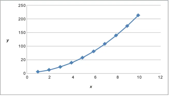
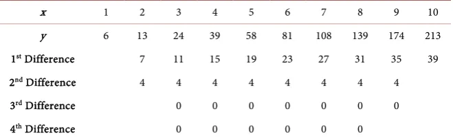
row, Table 1 shows the y-value outputs for the sequence of regularly spaced 𝑥𝑥-value inputs at points 1, 2,,10 shown on the 1st row. A plot of this data is
shown in Figure 1. The problem is to determine the order of the polynomial that can generate these outputs and to find its coefficients.
The remaining rows in Table 1 show the successive differences of the y-values. The fact that the 3rd difference row in Table 1 is composed of all zeros implies
that a quadratic polynomial best describes this data. In fact this data was gener-ated by the quadratic polynomial: 2
2 3
y= x + +x .
I assume throughout this paper that the data are sampled at regular intervals. Without loss of generality these intervals can be assumed to be of unit length. Then the following general observations can be made:
1) If the
(
)
st 1m+ difference row is all zero, then the data is best described by an mth order polynomial: 1
1 1 0
m m
m m
a x +a −x − ++a x+a
2) If the
(
)
st 1m+ difference row is all zero, then m a! m is the constant in the mth row. From this observation the coefficient of the highest term can be
found. For example in Table 1 since the 3rd difference row is all zero then
2 2!a is the constant in the 2nd difference row. Since this constant is 4, it immediately
follows that the highest term should be 2 2 4x 2!=2x
3) The lower order terms can be found successively by back substituting and subtracting the highest term. In this method, the data y in Table 1 is replaced by
y′ where m m
y′ = −y a x , and then reapplying the method of finite differences
[image:3.595.209.539.521.709.2]on the y′ data. Using this approach for the data in Table 1, one obtains the next term as follows:
DOI: 10.4236/ojs.2018.81005 52 Open Journal of Statistics In Table 2 the 2nd difference row is all zero. Hence
1
1!a is the constant in the 1st difference row. Since this constant is 1, the next highest term should be
1 1!x =x.
Again, the final term can be found by replacing y′ in Table 2 by y′′ where
1 1
m m y′′= −y′ a −x − :
The computation in Table 3 yields 3 as the constant term for the polynomial fit.
Hence, by successive applications of the finite difference method in this man-ner, the best fit polynomial to the 𝑦𝑦 data in Table 1 is found to be 2
2x + +x 3.
2. The Method of Finite Difference Regression
In this section I describe the Finite Difference Regression method, compare the results obtained from this method to those from classical regression, and show unbiasedness and consistency properties of the Finite Difference Regression coefficients.
[image:4.595.209.539.404.506.2]The intuitive idea behind the method of Finite Difference Regression is simple. Suppose one were to add normally distributed noise with mean 0 independently to each of the y-values for example in Table 1 to make them noisy, then unlike the non-noisy situation, one cannot expect all entries in a difference row to be all
Table 1. Finite Differences on y-value outputs for the sequence of regularly spaced
x-value inputs.
x 1 2 3 4 5 6 7 8 9 10 y 6 13 24 39 58 81 108 139 174 213 1st Difference 7 11 15 19 23 27 31 35 39
2nd Difference 4 4 4 4 4 4 4 4
3rd Difference 0 0 0 0 0 0 0
4th Difference 0 0 0 0 0 0
Table 2. Second iteration of finding terms to fit the model.
x 1 2 3 4 5 6 7 8 9 10 y 6 13 24 39 58 81 108 139 174 213
2
2
y′ = −y x 4 5 6 7 8 9 10 11 12 13
1st Difference 1 1 1 1 1 1 1 1 1
2nd Difference 0 0 0 0 0 0 0 0
Table 3. Final iteration of finding terms to fit the model.
x 1 2 3 4 5 6 7 8 9 10
y′ 4 5 6 7 8 9 10 11 12 13
y′′=y′−x 3 3 3 3 3 3 3 3 3 3
DOI: 10.4236/ojs.2018.81005 53 Open Journal of Statistics identically equal to zero. However, since differences between normally distri-buted random variables are also normally distridistri-buted (albeit with higher va-riance), each of the samples in a difference row (as in the rows of Table 1) would also be normally distributed with different means until one hits a difference row where the mean is zero with high probability. It is this highly probable ze-ro-mean row that should be the all zero difference row in the absence or elimi-nation of noise. The condition that the mean is zero with high probability can be objectively tested on each difference row using a t-test on the samples in that row, where the null hypothesis H0 tests for zero population mean and the
alter-native hypothesis Ha tests for non-zero population mean. This is the main idea
behind the method of Finite Difference Regression—the replacement of the no-tion of an all zero difference row in the non-noisy case by the nono-tion of a highly probable row of all zeros in the noisy case and usage of the statistical t-test to test for the zero population mean hypothesis.
2.1. Statistical Independence and Its Relation to the Degrees of
Freedom
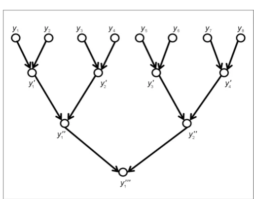
While it is true that successive differences will produce normally distributed samples, not all the samples so produced are statistically independent of one another. For example as shown in Figure 2, the noisy data samples y y y y1, 2, 3, 4 generate the next difference sequence y y y1′ ′ ′, 2, 3—not all of these values are in-dependent. Since y1′ and y2′ both depend upon the value of y2 they are not independent. Similarly, y2′ and y3′ are not independent because both depend upon y3. However, y1′ and y3′ having no point in common, are independent!
This observation can be generalized by the following process. Suppose I had K observations to begin with.If I were to produce successive differences by skip-ping over every other term, in the manner of a binary tree as shown in Figure 3, I would obtain independent normally distributed samples. Each level of the tree would have independent normally distributed finite differences denoted in Fig-ure 3 (shown with K=8) by y y′ ′′, , and so on. This method would retain all the properties of finite differences, in particular the highly probable zero mean row; plus it would have the added benefit of not having any dependent samples. If this method were implemented, and a t-test invoked at every level of the binary tree, then the number of samples in the test would be halved at each level, and consequently the degrees of freedom would be affected. In other words, if k denotes the number of samples3 at a particular level of the tree, then in the
next level one would get k/2 samples. Then according to the theory of t-tests, the degrees of freedom for the first level would be k−1, in the next level it would be
2 1
DOI: 10.4236/ojs.2018.81005 54 Open Journal of Statistics
Figure 2. Successive finite differences.
Figure 3. A binary tree of successive differences.
that at every stage the number of independent samples is halved and therefore the degrees of freedom is one less than this number.
2.2. An Example of Order Finding
Table A1 in Appendix 2 gives an example of how the Finite Difference Regres-sion method works to find the order of the best fitting polynomial. The 1st two
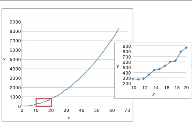
columns of Table A1 are the pivoted rows of Table 1. Independent zero-mean normally distributed random noise with standard deviation of 30.0 is generated in the 3rd column and added to the values of y in the 4th column. Thus, the 4th
column represents noisy values of the data y. A graph of this noisy data is shown in Figure 4. Finally, columns 5 through 9 represent successive finite differences from 1st to 5th, computed in the same way as in Table 1. The last 6 rows of Table
9 highlighted in yellow show the statistical computations associated with the method. These are described below in Section 2.3.
2.3. The Statistical Computations
[image:6.595.243.501.182.384.2]DOI: 10.4236/ojs.2018.81005 55 Open Journal of Statistics
Figure 4. Graph of the noisy data in Table 5 with insert showing magnified view for
10≤ ≤x 20.
Header titled n = Number of samples Header titled x = Sample mean
Header titled s = Sample standard deviation Header titled t = Test statistic = x x
s n s n
µ
−
= (substituting µ=0)
Header titled df = Degrees of freedom computed as detailed in Section 2.1 Header titled P-value = 2 Area to right of with given for 0
2 Area to left of with given for 0
t df t
t df t
× >
× <
2.4. Conclusions from the
t
-Test
One of the assumptions of the t-test is that the sample size n is large. Typically,
30
n≥ is required. This assumption is violated in some of the columns of Table
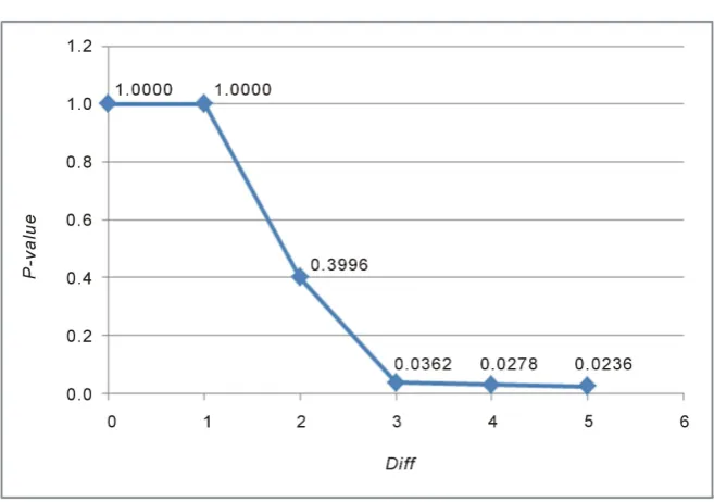
A1. However the table is merely for illustrative purposes. Even so, it shows the power of the method to correctly ascertain the order of the best fitting poly-nomial because one can hardly fail to notice the precipitous drop in P-value in the 3rd difference column (titled Diff 3). The plot in Figure 5 showing the
P-values of the 5 difference columns graphically displays this drop.
The insignificant P-value in the 3rd difference column implies that with high
probability the order of the best fitting polynomial should be m=2, i.e. a
qua-dratic polynomial is the best fit polynomial to the data in Table A1.
2.5. Comparison to Classical Regression
In classical polynomial regression, R2 values instead of P-values represent the
goodness of fit. Using Microsoft Excel’s built-in program to generate 2
R values
to polynomial fits, I generated Table 4 by restricting the highest degree m of the best fitting polynomial 1
1 1 0
m m
m m
a x +a −x − ++a x+a for the noisy data in
DOI: 10.4236/ojs.2018.81005 56 Open Journal of Statistics
[image:8.595.205.538.344.378.2]Figure 5. Graph of P-value vs. Diff.
Table 4.R2 values in classical regression as a function of degree m.
m 1 (Linear) 2 (Quadratic) 3 (Cubic) 4 5 R2 value 0.9403 0.9999 0.9999 0.9999 0.9999
Table 4 shows that the R2 values used in classical regression do not have the
sensitivity that the P-values with t-tests possess. The clear drop that occurs in the P-values as shown in Figure 5 does not have a corresponding sharp rise in R2
values in Table 4. Also, unlike classical regression which requires R2 values to be
fitted with every polynomial the Finite Difference Regression is a one-shot test that gives a clear estimate of the order of the best fitting polynomial by testing the significance of the probabilities (P-values). The first successive difference column whose P-value is less than the significance level (a belief threshold for the viable model) comes out to be the best fitting polynomial model.
Unlike classical regression, however, this method requires a large sample size n, preferably one that is a power of 2. Also, because the degrees of freedom get halved at each successive difference and the degrees of freedom have to remain positive, the highest order polynomial that can be fit by this method is of the or-der log2n. This is generally acceptable because the order of the best fitting po-lynomials should by definition be small constants. Other classical model order selection heuristics like AIC or BIC (see [3]) would also heavily penalize high order models.
2.6. Determining the Coefficients
DOI: 10.4236/ojs.2018.81005 57 Open Journal of Statistics in Section 1.
In the non-noisy situation described in Section 1, the matter was simple: there was a difference row of all zeros and therefore the previous difference row was a constant that could be used to determine the coefficient of the highest degree. In the noisy case, the issue is complicated because there is no such row that consists of all zeros and therefore the previous difference row is not a constant. However, the intuitive idea behind the method of Finite Difference Regression (see the 2nd
paragraph of Section 2), led me to assume that the sample mean x would be an
excellent choice for the previous difference row constant, since it is the unique number that minimizes the sum of squares of the residuals. From Table A1, the all zero column is the 3rd difference column, and therefore x=4.29 (the
sample mean of the 2nd difference column in Table A1) corresponds to the
constant difference. Thus as described in Section 1, the highest term should be
2 2
2! 2.145 x
x = x ; the next term determined from the sample mean of the
“con-stant” column after subtracting the values of the highest term yields −7.464x; and finally the constant term is 78.69. Thus ˆ 2
2.145 7.464 78.69
y= x − x+ is the
estimated polynomial model.
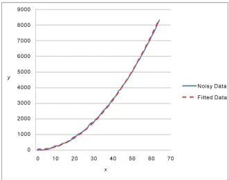
[image:9.595.207.539.428.689.2]Table A2 in Appendix 2 compares the noisy data to the best fit polynomial estimate using the method of successive finite differences. Note that the residuals are not very small; however, their average turns out to be −0.00078 indicating a good fit. The polynomial fit is overlaid on the noisy y data in Figure 6, in which the blue line shows the noisy data, and the dashed red line depicts the values of the estimated yˆ.
Figure 6. Graph of best fitting polynomial 2
ˆ 2.145 7.464 78.69
y= x − x+ overlaid on the
DOI: 10.4236/ojs.2018.81005 58 Open Journal of Statistics
2.7. Unbiasedness and Consistency of the Coefficient Estimates
In this section I prove that the coefficients estimated by the Finite Difference Regression method as detailed in Section 2.6 are unbiased and consistent. The properties of unbiasedness and consistency are very important for estimators (see [6] p. 393). The unbiasedness property shows that there is no systematic offset between the estimate and the actual value of a parameter. It is proved by showing that the mean of the difference between the estimate and the actual value is zero. The consistency property shows that the estimates get better with more observations. It is proved by showing that a non-zero difference between the estimate and the actual value becomes highly improbable with a large num-ber of observations. The analysis focuses on the estimate of the leading coeffi-cient i.e. that associated with highest degree because the asymptotic properties of the polynomial fit will be most sensitive to that value.Consider the following table that shows the symbolic formulas for the succes-sive differences for the n observationsy y1, 2,,yn:
For subsequent ease of notation, I introduce a change of variables def 1
i i
z = y+
for 0≤ ≤ −i n 1. With this renaming/re-indexing, Table 5 can be rewritten as
(note that the row indices have also changed):
For any m, 0≤ ≤ −m n 1, the mth Diff column consists of expressions in rows
indexed from m through n−1. Using mathematical induction, the mth Diff
column can be shown to be:
If the underlying polynomial is an mth order polynomial
( )
11 1 0
m m
m m
f x =a x +a −x − + + a x+a , then in the case of noiseless observations, every row of Table 7 evaluates to the constant m a! m. In particular, for the k
th
[image:10.595.207.539.487.588.2]row in the mth Diff column shown in Table 7 one gets:
Table 5. Successive differences for n observations y y1, 2,,yn.
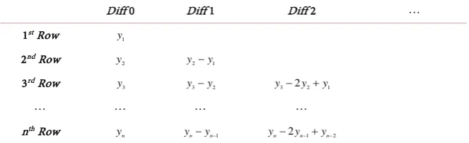
Diff 0 Diff 1 Diff 2
1st Row
1
y
2nd Row
2
y y2−y1
3rd Row
3
y y3−y2 y3−2y2+y1
nth Row
n
y yn−yn−1 yn−2yn−1+yn−2
Table 6. Changing yi+1 from Table 5 to zi for 0≤ ≤ −i n 1.
Diff 0 Diff 1 Diff 2
0th Row
0
z
1st Row
1
z z1−z0
2nd Row
2
z z2−z1 z2−2z1+z0
(n − 1)th Row
1 n
DOI: 10.4236/ojs.2018.81005 59 Open Journal of Statistics
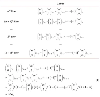
Table 7. The mth diff column.
Diff m
mth Row
( )
1 2 1 0
0 1 2
m
m m m
m m m m
z z z z
m
− −
− + + + −
(m + 1)th Row
( )
1 1 1 1
0 1 2
m
m m m
m m m m
z z z z
m + − − + + + −
kth Row
( )
1 2 1
0 1 2
m
k k k k m
m m m m
z z z z
m − − − − + + + −
(n − 1)th Row
( )
1 2 3 1 1
0 1 2
m
n n n n m
m m m m
z z z z
m − − − − − − + + + −
( )
( )
(
)
( )
(
)
( )
(
)
1 21 1 1
1
0 1 2
1
0 1 2
1 1 1 1
0 1 2
!
m
k k k k m
m
k k k k m
m
m
m m m m
z z z z
m
m m m m
y y y y
m
m m m m
f k f k f k f k m
m m a − − − + − + − − + + + − = − + + + − = + − + − + + − + − = (1)
In case of noisy observations, let each re-indexed observation z now be cor-rupted by a sequence of additive zero-mean independent identically distri-buted random variables N0,N1,,Nn−1, each with variance
2
σ . In other
words:
[ ]
2 20 and f ro 0 i = i=σ ≤ <i n
N N
[ ]
0 for0i j i j i j n
= = ≤ < < N N N N
where
[ ]
denotes the expectation operator. (See for example [7] pp. 220-223.) This addition of random variables makes the z’s also random variables de-noted now asZ
, and so Zi= f i(
+ +1)
Ni for 0≤ <i n. In this case, the kthrow in the mth Diff column shown in Table 7 is the random variable
k
R where:
( )
( )
(
)
( )
(
)
( )
(
)
1 2 1 2 1 10 1 2
1
0 1 2
1 1 1 1
0 1 2
0 1 2
m
k k k k k m
m
k k k k m
m
k k
m m m m
m
m m m m
m
m m m m
f k f k f k f k m
m
m m m
N − − − − − − − = − + + + − = − + + + − + + − + − + + − + − = − +
R Z Z Z Z
N N N N
N
( )
2 1 !
m
k k m m
m m a m − − + + − +
N N
DOI: 10.4236/ojs.2018.81005 60 Open Journal of Statistics where, the last step of Equation (2) follows from the identity in Equation (1).
Let the random variable ˆ
( )
m nA denote the estimate of am with the n ob-servations. Then as described in Section 2.6, since there are
(
n−m)
rows in themth Diff column, the sample mean of the R’s divided by m! provides the
re-quired estimate. In other words,
( )
(
1)
1ˆ ! n m k k m n
m n m
−
= =
−
∑
A R (3)
Now, define the reduced row random variable Qk for the m
th Diff column
shown in Table 7 as: def
! for 1
k = k−m am m≤ ≤ −k n
Q R (4)
Then, substituting back into Equation (3):
( )
(
)
(
)
(
)
(
(
)
)
(
)
1 1 1 1 1 1 ˆ ! ! ! ! 1 ! ! 1 ! n nm k m
k m k m
n m k k m n k m k m
n m a
m n m m n m
m a n m
m n m m n m
a
m n m
− − = = − = − = = + − − − = + − − = + −
∑
∑
∑
∑
A Q Q QWhich, upon rearranging yields:
( )
(
1)
1ˆ
!
n
m m k
k m
n a
m n m
−
=
− =
−
∑
A Q (5)
Note that it is the statistics of the expression ˆ
( )
m n −amA on the left-hand
side of Equation (5) that will prove the properties of unbiasedness and consis-tency of the estimate ˆ
( )
m n
A . Also note that by definition (4) and from
Equa-tion (2), the reduced row random variable Qk for the m
th Diff column can be
explicitly written as:
( )
1 2 1
0 1 2
m
k k k k k m
m m m m
Q
m
− − −
= − + + + −
N N N N (6)
2.7.1. Result 1: ˆ
( )
m
A n Is an Unbiased Estimate of am
Taking the expectation operator
[ ]
on both sides of Equation (6):[ ]
( )
[ ]
[
]
( )
[
]
1 2
1
1
0 1 2
1 0
0 1
m
k k k k k m
m
k k k m
m m m m
m
m m m
m − − − − − = − + + + − = − + + − =
Q N N N N
N N N
(7)
The last step in Equation (7) follows from the fact that the random variables
i
N are all zero-mean. Then, taking the expectation operator on both sides of
Equation (5), and using the result from Equation (7):
( )
(
1)
1[ ]
ˆ 0
!
n
m m k
k m
n a
m n m
−
=
− = =
A −
∑
QDOI: 10.4236/ojs.2018.81005 61 Open Journal of Statistics Hence, ˆ
( )
0m n am
− = A
for all n. This proves the unbiasedness property of ˆ
( )
m n
A .
∎
2.7.2. Result 2: ˆ
( )
m
A n Is a Consistent Estimate of am
Since the random variable ˆ
( )
m n −amA has been shown to be of zero-mean by
virtue of its unbiasedness property, the variance of this random variable is simply
(
ˆ( )
)
2m n am
−
A
. I show the consistency property of the estimate
( )
ˆ m n
A by way of deriving an upper-bound for
(
ˆm( )
n am)
2 −
A
and
show-ing that this upper-bound vanishes to 0 in the limit n→ ∞.
Writing out the reduced row random variables Qk for each row k for the mth Diff column from Equation (6) one gets the following series of
(
n−m)
equa-tions:
( )
1 2 1 0
0 1 2
m
m m m m
m m m m
m
− −
= − + + + −
Q N N N N
( )
1 1 1 1 1
0 1 2
m
m m m m
m m m m
m
+ + −
= − + + + −
Q N N N N
( )
1 2 1
0 1 2
m
k k k k k m
m m m m
m
− − −
= − + + + −
Q N N N N
( )
1 1 2 3 1 1
0 1 2
m
n n n n n m
m m m m
m
− − − − − −
= − + + + −
Q N N N N
Summing up these
(
n−m)
equations column by column:( )
1
1 2 3 1
1 2 1 0
0 1 2
n
m
n n n n m
k m m m
k m
m m m m
m − − − − − − − − = = − + + + −
∑
Q S S S S (9)where for
(
n− −1 m)
≤ ≤i(
n−1)
and 0≤ ≤j m define:def i i
j k
k j=
=
∑
S N (10)
Squaring both sides of Equation (10), and then taking expectations:
( )
[
]
(
)
(
)
2 2 22 2 2
1
i i
i
j k k
k j k j
i i
k
k j k j
i j σ σ = = = = = = + = + = = − +
∑
∑
∑
∑
S N N
N SCT SCT (11)
In Equation (11) I have invoked the zero-mean, independent nature of the N’s to cause the “sum of cross-terms” term SCT to vanish.
Define a new sequence of
(
m+1)
random variables T T0, 1,,Tm as follows:( )
def 1
1i n i for 0
i m i
m i m i − − − = − ≤ ≤
DOI: 10.4236/ojs.2018.81005 62 Open Journal of Statistics By squaring both sides of definition (12), and then taking expectations:
( )
2 2(
)
2 2(
)
2 2(
)
2 1 1 2
1 i n i n i
i m i m i
m m m
n m
i i i σ
− − − − − − = − = = −
T S S
(13)
where, the final step in Equation (13) follows from Equation (11). Using definition (12), Equation (9) can be rewritten as:
1 0 1 n k m k m − = = + + +
∑
Q T T T (14)Then as
(
)
2(
)
(
2 2 2)
0 1 m m 1 0 1 m
+ + + ≤ + + + + T T T T T T
(see
Appendix 1, squaring both sides of Equation (14), and then taking expectations:
(
)
(
)
(
)
(
)(
)
( )
(
)(
)
[ ]
2 1
2 2 2 2
0 1 0 1
2 2 2
2
2
1
1 From Equation 13
[From binomial ident
0 1
2
1 ity (see 8 pg.
n
k m m
k m
m
m m m
m n m
m
m
m n m
m σ σ − = = + + + ≤ + + + + = + − + + + = + −
∑
Q T T T T T T
64)]
(15) Finally, by squaring both sides of Equation (5), and then taking expectations I obtain the following inequality from inequality (15):
( )
(
)
( ) (
)
1 2(
( ) (
)( )
)
22
2 2 4
1 2 !
1 ˆ
! !
n
m m k
k m
m m
n a
m n m m n m
σ − = + − = ≤
A −
∑
Q − (16)
where, the last step in (16) is a rewriting of the binomial coefficient 2m
m
in
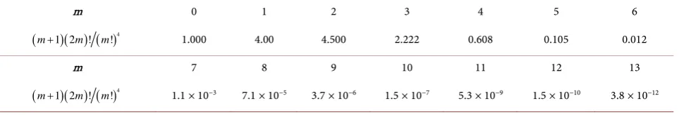
terms of factorials and subsequent simplification. It can be seen that the factor
(
)( ) ( )
41 2 ! !
m+ m m on the right hand side of inequality (16) is a super-exponentially decreasing function of m (above a con-stant) due to presence of the large
( )
4!
[image:14.595.206.541.77.366.2]m factor in its denominator. This factor is evaluated for a few values of m in Table 8.
Table 8 shows that:
( )
(
)
2(
)
24.5 ˆ
m n am
n m
σ
×
− ≤
A −
(17)
For the Finite Difference Regression method, m≤log2n (see Section 0 and the comments in Section 0). Thus, the right-hand-side denominator
2 log
n− ≥ −m n n in inequality (17) and therefore,
( )
(
)
2(
2)
2 4.5 ˆ
log
m n am
n n
σ
×
− ≤
A −
(18)
Taking limits on both sides of inequality (18),
( )
(
)
2(
2)
2 4.5 ˆ
lim lim 0
log
m m
n n a n n n
σ
→∞ →∞
×
− ≤ =
A −
DOI: 10.4236/ojs.2018.81005 63 Open Journal of Statistics
Table 8. The factor
(
)( ) ( )
41 2 ! !
m+ m m evaluated for a few values of m.
m 0 1 2 3 4 5 6
( )( ) ( )4
1 2 ! !
m+ m m 1.000 4.00 4.500 2.222 0.608 0.105 0.012
m 7 8 9 10 11 12 13
( )( ) ( )4
1 2 ! !
m+ m m 1.1 × 10⁻³ 7.1 × 10⁻⁵ 3.7 × 10⁻⁶ 1.5 × 10⁻⁷ 5.3 × 10⁻⁹ 1.5 × 10⁻¹⁰ 3.8 × 10⁻¹²
However, as
(
ˆ( )
)
2 0m n am
− ≥
A
, inequality (19) implies that:
( )
(
)
2ˆ
lim m m 0
n→∞ n a
− =
A
(20)
Then invoking Chebyshev’s inequality (see [7] p. 233, [9] p. 151) yields:
( )
(
( )
)
2
2 ˆ lim ˆ
lim 0, for any 0
m m
n
m m
n
n a
Prob n a ε ε
ε
→∞ →∞
−
− > ≤ = >
A A
This proves the consistency property of ˆ
( )
m nA .
∎
2.7.3. A Note on the Asymptotic Properties of the Fit
Inequality (16) and the values in Table 8 show that the higher the degree m of the polynomial, the lower is the variance of the estimate of its leading coefficient. This excellent property implies that the asymptotic properties of the fit (that are most sensitive to this leading coefficient) are stable, in the sense that the value of the asymptote becomes less varying with increasing degrees of the fitting poly-nomial.
3. Conclusions and Further Work
In this paper I have presented a novel polynomial regression method for un-iformly sampled data points called the method of Finite Difference Regression. Unlike classical regression methods in which the order of the best fitting poly-nomial model is unknown and is estimated from the R2 values, I have shown
how the t-test can be combined with the method of finite differences to provide a more sensitive and objective measure of the order of the best fitting polynomi-al. Furthermore, I have carried forward the method of Finite Difference Regres-sion, reemploying the finite differences obtained during order determination, to provide estimates of the coefficients of the best fitting polynomial. I have shown that not only are these coefficients unbiased and consistent, but also that the asymptotic properties of the fit get better with increasing degrees of the fitting polynomial.
At least three other avenues of further research remain to be explored:
DOI: 10.4236/ojs.2018.81005 64 Open Journal of Statistics 2) The classical regression methods work on non-uniformly sampled data sets. Extending this method to non-uniformly sampled data should be possible.
3) Automatically finding a good t-test significance level i.e. the precipitously low P-value that sets the order of the best fitting polynomial (as described in Section 2.4) remains an open problem. For this, heuristics in the spirit of AIC or BIC methods (see [3]) in the classical case may perhaps be required.
Acknowledgements
I thank Prof. Brad Lucier for his interest and for the helpful discussions and comments that made this a better paper. I am also grateful to Dr. Jan Frydendahl for encouraging me to pursue this research activity.
References
[1] Gauss, C.F. (1857) Theory of the Motion of the Heavenly Bodies Moving about the Sun in Conic Sections. Davis, C.H., Trans., Little, Brown & Co., Boston, MA. [2] Peck, R., Olsen, C. and Devore, J. (2005) Introduction to Statistics and Data
Analy-sis. 2nd Edition, Thomson Brooks/Cole, Belmont, CA.
[3] Burnham, K.P. and Anderson, D.R. (2004) Multimodel Inference: Understanding AIC and BIC in Model Selection. Sociological Methods and Research, 33, 261-304.
https://doi.org/10.1177/0049124104268644
[4] Newton, I. (1848) Newton’s Principia: The Mathematical Principles of Natural Phi-losophy. Motte, A., Trans., Daniel Adee, New York.
[5] Hämmerlin, G. and Hoffmann, K.-H. (1991) Numerical Mathematics. Schumaker, L.L., Trans., Springer, New York.https://doi.org/10.1007/978-1-4612-4442-4
[6] Cover, T.M. and Thomas, J.A. (2006) Elements of Information Theory. 2nd Edition, John Wiley & Sons, Inc., New York.
[7] Feller, W. (1968) An Introduction to Probability Theory and Its Applications. 3rd Edition, Vol. I, John Wiley & Sons, Inc., New York.
[8] Tucker, A. (1980) Applied Combinatorics. John Wiley & Sons, Inc., New York. [9] Feller, W. (1971) An Introduction to Probability Theory and Its Applications. 2nd
Edition, Vol. II, John Wiley & Sons, Inc., New York.
[10] Student (1908) The Probable Error of a Mean. Biometrika, 6, 1-25.
DOI: 10.4236/ojs.2018.81005 65 Open Journal of Statistics
Appendix 1
To show that for any sequence of
(
m+1)
random variables T T0, 1,,Tm:(
)
2(
)
(
2 2 2)
0 1 m m 1 0 1 m
+ + + ≤ + + + + T T T T T T
The proof follows from a variance-like consideration. Given the random variables T T0, 1,,Tm and any ran-dom variable T, the sum of squares randomvariable
∑
im=0(
Ti−T)
2 is always non-negative. Its expected value(
)
20 m i i= −
∑
T T is therefore always non-negative. Choosing the random variable def
(
)
0 1
m i
i= m
=
∑
+T T i.e. the
“mean” of T T0, 1,,Tm proves the inequality as follows:
(
)
(
)
(
)
(
)
(
)
2 0 2 2 0 2 20 0 0
2 2
0 0 0
2 2 0 0 2 2 2 1
2 1 1 from defn. of
m i i m i i i
m m m
i i
i i i
m m m
i i
i i i
m i i T m m = = = = = = = = = ≤ − = − + = − + = − + = − × + + × +
∑
∑
∑
∑
∑
∑
∑
∑
∑
T TT TT T
TT T
T T T T
T T T T T
(
)
(
)
(
)
(
)
(
)
(
)
(
)
(
)
2 2 2
0 2 2 0 2 2 0 0 2 2 0 1 2 0
2 1 1
1
1 from defn. of
1 1 1 m i i m i i m m i i i i m i m i m m m m m m m = = = = = = − + + + = − + = − + + + = − + + + +
∑
∑
∑
∑
∑
T T T
T T
T
T T
T T T T
Multiplying both sides of the above inequality by
(
m+1)
and rearranging yields the required result.DOI: 10.4236/ojs.2018.81005 66 Open Journal of Statistics
Appendix 2
Table A1. Example showing how the finite difference regression method works.
x y Noise y + Noise Diff 1 Diff 2 Diff 3 Diff 4 Diff 5
1 6 −3.46 2.54
2 13 11.08 24.08 21.53
3 24 −10.78 13.22 −10.86 −32.39
4 39 −12.23 26.77 13.55 24.41 56.81
5 58 −15.22 42.78 16.01 2.46 −21.95 −78.76
DOI: 10.4236/ojs.2018.81005 67 Open Journal of Statistics Continued
36 2631 15.10 2646.10 125.79 −34.59 −43.86 −34.70 −23.92 37 2778 10.35 2788.35 142.24 16.45 51.04 94.91 129.60 38 2929 −14.74 2914.26 125.91 −16.33 −32.79 −83.83 −178.74 39 3084 39.17 3123.17 208.91 83.00 99.33 132.12 215.95 40 3243 36.96 3279.96 156.80 −52.12 −135.12 −234.45 −366.57 41 3406 −4.73 3401.27 121.31 −35.49 16.63 151.74 386.19 42 3573 −6.60 3566.40 165.13 43.82 79.31 62.68 −89.06 43 3744 65.08 3809.08 242.68 77.55 33.74 −45.57 −108.25 44 3919 −22.02 3896.98 87.90 −154.77 −232.33 −266.06 −220.49 45 4098 13.68 4111.68 214.70 126.80 281.57 513.90 779.96 46 4281 −6.64 4274.36 162.67 −52.03 −178.82 −460.39 −974.29 47 4468 −5.14 4462.86 188.50 25.83 77.86 256.68 717.07 48 4659 −37.01 4621.99 159.13 −29.37 −55.20 −133.06 −389.74 49 4854 6.42 4860.42 238.43 79.30 108.67 163.88 296.94 50 5053 −46.83 5006.17 145.75 −92.68 −171.98 −280.66 −444.53 51 5256 7.28 5263.28 257.11 111.36 204.04 376.03 656.68 52 5463 −8.25 5454.75 191.47 −65.64 −177.00 −381.04 −757.07 53 5674 18.11 5692.11 237.36 45.89 111.53 288.53 669.57 54 5889 −20.01 5868.99 176.89 −60.48 −106.37 −217.90 −506.42 55 6108 5.34 6113.34 244.35 67.46 127.94 234.30 452.20 56 6331 1.67 6332.67 219.33 −25.02 −92.48 −220.42 −454.72 57 6558 8.07 6566.07 233.40 14.07 39.09 131.58 351.99 58 6789 7.01 6796.01 229.94 −3.46 −17.54 −56.63 −188.21 59 7024 −6.75 7017.25 221.24 −8.69 −5.23 12.31 68.94 60 7263 14.76 7277.76 260.51 39.27 47.96 53.19 40.88 61 7506 −18.95 7487.05 209.29 −51.22 −90.48 −138.44 −191.63 62 7753 −2.33 7750.67 263.61 54.32 105.54 196.03 334.47 63 8004 24.70 8028.70 278.03 14.42 −39.91 −145.45 −341.47 64 8259 57.11 8316.11 287.41 9.38 −5.04 34.87 180.32
n 64 63 62 61 60 59
x 2833.75 131.96 4.29 0.68 −1.03 1.93
s 2517.12 83.47 63.10 113.72 211.20 399.59
t 9.01 12.55 0.54 0.05 −0.04 0.04
df 63 31 15 7 3 1
DOI: 10.4236/ojs.2018.81005 68 Open Journal of Statistics
Table A2. The noisy data compared to the best fit polynomial estimate 2
ˆ 2.145 7.464 78.69
y= x − x+ determined from the
successive finite differences method.
x y + Noise ˆy Residual x y + Noise ˆy Residual
[image:20.595.58.539.106.720.2]