A Tractable Approach to Base Station Sleep Mode Power Consumption and Deactivation Latency

A Tractable Approach to Base Station Sleep

Mode Power Consumption and Deactivation

Latency

Oluwakayode Onireti

, Abdelrahim Mohamed

, Haris Pervaiz

and Muhammad Imran

†_{Institute for Communication Systems ICS, University of Surrey, Guildford, UK}

Email: oluwakayode.onireti@glasgow.ac.uk

Abstract—We consider an idealistic scenario where the vacation (no-load) period of a typical base station (BS) is known in advance such that its vacation time can be matched with a sleep depth. The latter is the sum of the deactivation latency, actual sleep period and reacti-vation latency. Noting that the power consumed during the actual sleep period is a function of the deactivation latency, we derive an accurate closed-form expression for the optimal deactivation latency for deterministic BS vacation time. Further, using this expression, we derive the optimal average power consumption for the case where the vacation time follows a known distribution. Numerical results show that significant power consumption savings can be achieved in the sleep mode by selecting the optimal deactivation latency for each vacation period. Furthermore, our results also show that deactivating the BS hardware is sub-optimal for BS vacation less than a particular threshold value.

I. INTRODUCTION

A breakdown of the power consumption of the cellular networks reflects that about 80% of the total power is consumed by the base stations (BSs) [1]. Hence, most optimization effort towards maintaining power consumption evolution in the fifth generation (5G) cellular networks has been on the BS. An accurate power consumption model (PCM) is a prerequisite for such optimization. In [2], the authors presented a linear PCM for the BS in the active state. The PCM for a BS on no-load and sleep mode has been considered in [3]. However, only one sleep mode has been considered in the latter work. In [4], [5], the authors identified four different sleep modes with different power savings based on the BS’s hardware capability. Each sleep mode is associated with a given duration; all the BS sub-components that can enter and exit the sleep mode fast enough are considered sleeping in that mode, while the subcomponents having a longer latency are considered to be still active. In other words, each sleep mode is characterized by a sleep depth (duration) which is the sum of the subcomponent deactivation and reactiva-tion latencies and the actual sleep period. The power saving at each sleep mode is attributed to the actual sleep period [4]. Moreover, the power consumed during subcomponent reactivation and deactivation processes exceeds that of the actual sleep period and in particular,

2EMHFWWUDIILF GXUDWLRQSUHGLFWLRQ

HVWLPDWLRQ %6YDFDWLRQ WLPHHVWLPDWRU 2EMHFWQDUULYDO

WLPHVWDPS

&DSWXUHG REMHFWVL]H OHQJWK DUULYDO WLPHVWDPS

2EMHFWQWUDIILF JHQHUDWLRQSKDVH

2QD 2QD 2QD 2QS 2QS

2EMHFWPRELOLW\DQGSDWK GHWDLOV

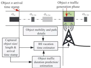
Fig. 1: Estimating the BS vacation and operational time in a single-queue single-server system

the no-load power consumption [6], [7].

The relaxed constraints for BS on/off operation in the control and data separation architecture [8], [9], which is a candidate architecture for 5G networks [10], means accurate modeling of the sleep mode is essential when evaluating the energy saving gains of this architecture. Accurate evaluation of such gains can only be attained by selecting the optimal sleep depth, i.e., selecting the optimal subcomponent deactivation and reactivation latency for each BS vacation period. The latter refers to the time interval at which the BS is not loaded with data and it is also referred to as the no-load interval. In this paper, we assume that the vacation period of a typical BS is known in advance and that it can be matched with the sleep depth, which mini-mizes the average power consumption. Furthermore, we consider that the reactivation and deactivation latencies to be proportional. Hence, we propose here the optimal deactivation latency for a BS. Though the knowledge of the vacation is not trivial in a typical cellular network, this assumption is valid for some fixed rate single-queue single-server system such as depicted in Fig. 1 1_.

1_{In this figure, 1) the time stamp of the object arrival to the system}

In [11], using the time-triggered four sleep modes defined in [4], [5], the authors evaluated the impact of sleeping BS on the overall BS energy consumption. Their results for 4G showed an energy saving gains up to 22% due to the limited set of sleep modes available for use. In [12], the authors utilized a curve fitting function to approximate the sleep mode power consumption as a function of the sleep depth. However, little insight could be gained from the analysis due to the high complexity of the approximated function. In this paper, we have followed a tractable approach, which gives more analytical insight, by considering an exponential decay of the actual sleep mode power consumption with subcomponent deactivation latency. Using the developed model, we evaluate the energy saving gain over the discrete four sleep state in [4], [5], [11].

The rest of this paper is organized as follows. We first discuss the network model in Section II, which includes the formulation of the power consumption in the actual sleep phase, the relationship between the re-activation and dere-activation latency and, the power con-sumption in the BS deactivation and reactivation phases. Using this network model in Section III, we accurately obtain the closed-form expression for the deactivation latency that minimizes the average power consumption for a deterministic BS vacation time. Relying on the closed-form expression we provide analytical insights and numerical results in Section IV. Our analysis reveals that deactivating the BS hardware is sub-optimal for BS vacation less than a particular threshold value. Beyond this threshold, increasing the BS vacation time leads to a reduction in the sleep mode power consumption. Conclusions are drawn in Section V.

II. NETWORKMODEL

We consider a network where the vacation times of a typical BS are known in advance. In such a network, the ith _{vacation time τ}

i of a typical BS can

be rightly matched with the sleep depth that achieves maximum energy savings. The BS’s sleep depth during the ith _{vacation period is made up of the}

compo-nent/subcomponent2 _{deactivation latencyτ}

di, the actual

sleep period τsi, and the subcomponent reactivation

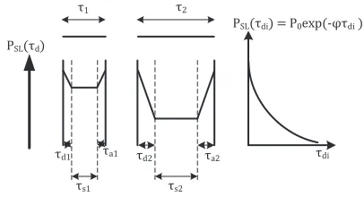
latencyτai, as illustrated in Fig. 2. We consider that the

vacation time of a typical BS follows a deterministic or uniform distribution. We aim to obtain the power savings gain that can be achieved as a result of the op-timal matching of the sleep depth with the BS vacation time. In order to achieve this, we first present the power consumption at the various phases of the sleep depth.

A. Power Consumption in the Actual Sleep Phase

We assume that subcomponents deactivation are done such that subcomponents with short deactivation times3 are the first to be deactivated. Increasing the BS

2_{The terms component and subcomponent are used interchangeably} 3_{Note that each subcomponent deactivation time is matched to a}

corresponding reactivation time

ɒ†ʹ

ɒ†ͳ ɒƒͳ ɒƒʹ

ɒʹ ɒͳ

ɒ•ʹ ɒ•ͳ

ሺɒ†ሻ

ɒ†‹ ሺɒ†‹ሻൌͲ‡š’ሺǦɔɒ†‹ሻ

Fig. 2: Base station transition latency showing, subcompo-nent deactivation latency, actual sleep period and reactivation latency. PSL is the power consumed by the BS during the

actual sleep period.

deactivation latency implies deactivating more subcom-ponents, and hence, a reduction in the power consumed during the actual sleep phase, as illustrated in Fig. 2. This remains the case until when the deepest sleep level, where no further deactivation of subcomponents is possible, has been attained. Hence, in this work, we model the power consumed in the actual sleep state as a function of the deactivation latency. The power consumed at the actual sleep state during the ith

vacation with deactivation latency τdi can be modeled

as

PSLi(τdi) =

P0exp (−ψτdi) 0≤τdi≤τd,max

P0exp (−ψτd,max) τdi > τd,max

(1) while assuming an exponential decay of the actual sleep mode power consumption with the subcomponent deactivation latency. The parameters ψ, P0 andτd,max

are the decay constant, no-load power consumption and maximum deactivation latency, respectively.

B. Deactivation and Reactivation Latencies

Measurement results in [13] have shown that the reactivation latencies of a typical BS’s subcomponents always exceed the corresponding deactivation latencies. Hence, we consider that theith _{reactivation latencyτ}

ai

and the corresponding deactivation latencyτdi are such

that

ηi=

τai

τdi

, (2)

where ηi > 1, ∀i. Furthermore, for the shortest sleep

depth in the long term evolution (LTE) network (71µs which is equivalent to one OFDM symbol), the small signal blocks considered for deactivation have to show a deactivation latency shorter than one-fourth of the sleep-depth, i.e.,17µslimit defined in [14] for the transmitter transient period [13]. This applies to the reactivation latency as well. By following the same reasoning, we assume that the actual sleep period during the ith

vacation period always exceeds the sum of the deac-tivation and reacdeac-tivation latencies, i.e.τsi≥(τdi+τai).

Consequently, the deactivation latency is bounded by

C. Deactivation and Reactivation Power Consumption

The power consumption during subcomponents re-activation is much greater than the no-load power con-sumption [6], [7]. Hence, following a similar assump-tion in [15] we model the power consumed during the reactivation phase as

Pτai =θ(2P0−PSLi(τdi)), (4) where θ ≥ 1 is a system defined parameter and P0

is the no-load power consumption. Pτai is a function of the actual sleep period power consumption and it increases with τdi, since higher τdi implies that more

subcomponents will be deactivated and hence a higher reactivation power consumption. For the deactivation power consumptionPτdi, we consider it to be a function of the average power consumed over the period of changing from no-load till when the actual sleep level has been attained. Hence, we modelPτdi as

Pτdi=ω(P0+PSLi(τdi)), (5) while assuming a linear decrease in power consumption over this period, where ω ≥ 1₂ is a system defined parameter.

III. OPTIMALAVERAGEPOWERCONSUMPTION A. Average Power Consumption

Given that the ith BS vacation period is matched to a sleep depth, the power consumed during the ith

vacation period, i.e., Ei can be expressed from [15] as

follows

E_i= τdiPτdi+τsiPSLi+τaiPτai

τi

, (6)

where the first, second and third terms of the numerator are the energy consumed during the BS deactivation, actual sleep and BS reactivation phases, respectively. The terms PSLi, Pτai and Pτdi can be expressed as a function of the subcomponent deactivation latency as in (1), (4) and (5), respectively. Furthermore, the reactiva-tion latency can also be expressed as a funcreactiva-tion of the deactivation latency as in (2). Given the deterministic vacation periodτi, the actual sleep period τsi can also

be expressed as a function of the deactivation latency such that

τsi=τi−(ηi+ 1)τdi, (7)

where ηi = η, ∀i, without loss of generality.

Conse-quently, the average power consumption during theith

vacation can be further expressed from (6) as

E_i(τdi, τi) =

1 τi

τdiPSL(τdi)[ω−η(θ+ 1)−1]

+τiPSL(τdi) +τdiP0(2ηθ+ω)

. (8)

B. Optimal Deactivation Latency

The optimal power consumption during the ith

vacation period can be obtained by finding τ⋆ di that

minimizes the power consumption expression in (8). Clearly,E_i(τdi)as defined in (8) is differentiable over its

domain, i.e. for τdi ∈[0, τd,max], when the actual sleep

levelPSL(τdi)is as defined in (1) such that ∂ E_i(τdi)

∂τdi can be expressed after simplification as

∂Ei(τdi)

∂τdi

= P0 τi

h

e−ψτdi_(Q

1−ψτi)−ψτdiQ1e−ψτdi

+ 2ηθ+ωi, (9) where P0

τi > 0 and Q1 = ω −η(θ + 1) −1. Let

τ⋆

di be the solution the equation

∂E_i(τdi)

∂τdi = 0. Then ∂E_i(τdi)

∂τdi ≤ 0 and

∂E_i(τdi)

∂τdi ≥ 0 for any τdi ∈ [0, τ ⋆ di]

and[τ⋆

di, τdi,max], respectively, which in turn means that E_i decreases over τdi ∈ [0, τdi⋆] and increases over

[τ⋆

di, τdi,max]. Consequently, for theithvacation period, Ei has a unique minimum, which occurs at τdi = τdi⋆.

Setting ∂Ei(τdi)

∂τdi = 0 in (9), we obtain that

g(τ_di⋆) =−(2ηθ+ω)eψτdi⋆ +Q₁ψτ⋆

di=Q1−ψτ,

(10) which can be solved in a straightforward manner by means of the Lambert W function, such that

τ_di⋆ = max

min

1 ψ

−W0

−(2ηθ+ω) Q1

e

1−ψτi

Q1

+ 1−ψτi

Q1

, τd,max

,0

, (11)

sinceτ⋆

di∈[0, τd,max]. Consequently, the optimal power

consumption during theith_{vacation can be obtained by}

substitutingτ⋆

di obtained from (11) into (8) such that

Ei(τdi⋆, τi) =

1 τi

τ_di⋆PSL(τdi⋆)(ω−η(θ+ 1)−1)

+τ PSL(τdi⋆) +τdi⋆P0(2ηθ+ω)

. (12)

C. Optimal Average Power Consumption

Moreover, given that the vacation time τ is uni-formly distributed in [τmin, τmax] such that f(τ) =

1

τmax−τmin, the optimal average power consumption can be expressed as

E_Av⋆ = Eτ[E(τd⋆, τ)]

= 1

τmax−τmin

Z

E(τ_d⋆, τ) dτ, (13) where τ⋆

d is obtained be replacing τi with τ in (11).

Since τ⋆

d is defined by the maxandminoperators, we

further expand the expression in (13) as

E_Av⋆ = 1

τmax−τmin

Z eτ

e τmin

P0 dτ+

Z τb

e τ

E(τ, τ_d⋆) dτ

+

Z τmax

b τ

E(τ, τd,max) dτ

!

where the parametersτeandτbare obtained by solving for τ in (11) that achieves τ⋆

d = 0 and τd⋆ = τd,max,

respectively, andeτmin= min(τmin,eτ). The parameters

e

τ andτ_bare subsequently defined as

e

τ =Q1 ψ

1 + 2ηθ+ω Q1

(15)

and

b

τ= Q1 ψ

1−ψτd,max+2

ηθ+ω Q1

eψτd,max

, (16)

respectively.

IV. ANALYTICALINSIGHTS ANDNUMERICAL RESULTS

A. Analytical Insights

1) Effect of increasing the vacation time τ on the optimal deactivation latency: Here we consider the scenario where the parameter θ = 1 and ω = 0.5 in (11). AsQ1=−2η−0.5so −_Qψτ₁ =_2ηψτ_+0.5. We assume

that the optimal deactivation latency is unbounded, such that the optimal deactivation latency can be expressed from (11) as

τ_di⋆=1 ψ

−W0

exp

1+ ψτ 2η+ 0.5

+ 1+ ψτ 2η+ 0.5

.

(17) Noting that ifz=W0[zexp(z)], thenz > W0[exp(z)].

Consequently,1 +_2ηψτ_+0.5 > W0

h

exp1 +_2ηψτ_+0.5iin (17), and 1 + ψτ

2η+0.5 dominates the latter expression.

Hence, increasing the vacation time leads an increase in the optimal deactivation latency.

2) Effect of increasing the reactivation/deactivation ratio η on the optimal deactivation latency: Increas-ingη implies increasing the subcomponent reactivation time. Following the earlier reasoning, it can be observed from (17) that for a fixed vacation time τ, and for

ω = 0.5 and θ = 1, increasing η leads to a decrease in the optimal subcomponent deactivation time. This is due to the higher power consumption during the subcomponent reactivation process as compared with the deactivation process.

3) Fixed power consumption in deactivation and reactivation: Given that the power consumption during the subcomponent deactivation and reactivation is fixed to Pτdi =Pτai =βP0, where β ≥1. The unbounded optimal deactivation latency can be expressed as

τ_di⋆ = 1 ψ

−W0

βexp

1 + ψτ η+ 1

+ 1 + ψτ η+ 1

(18) after following the same approach as in III-B. It can be seen from (18) that for a fixedψ, ηandτ, increasingβ

will lead to a reduction in τ_di⋆ and hence deeper sleep level will not be attainable. This implies that research on technologies related to a reduction in the power consumed during the subcomponent deactivation and reactivation processes should be embraced.

0 2 4 6 8 10

Vacation time,τi(s) 0

0.2 0.4 0.6 0.8 1 1.2

O

p

ti

m

al

d

ea

ct

iv

at

io

n

la

te

n

cy

,

τ

⋆ di

(s

)

η= 1,θ= 1, ω= 0.5

η= 2,θ= 1, ω= 0.5

η= 2,θ= 2, ω= 1

η= 1,β= 1 (fixed)

η= 2,β= 1 (fixed)

η= 2,β= 2 (fixed) Simulation

τi(s)

10-4

10-2

71.4µs 1 s

τ⋆ di

Fig. 3: Optimal deactivation latency as a function of deter-ministic BS vacation time.

B. Numerical Results

In this section, we present some numerical results to illustrate our analytical findings. The system parameters are as follows: P0= 139 W [4], [5],ψ= 2, τdi,max=

2 s.

In Fig. 3, we plot the optimal deactivation latency as a function of deterministic BS vacation time τi, for

η = 1,2, while considering the following scenarios 1) the subcomponents reactivation and deactivation power consumption are a function of the attained sleep level as defined in (4) and (5), respectively, 2) the power consumption during the subcomponents deactivation and reactivation processes are fixed to βP0, where

β > 1. Note that the magnified section in the figure shows the optimal deactivation latency for vacation time [71.4 µs,1 ms,10 ms,0.5 s,1 s]. It can be seen that for a fixedη, the optimal deactivation latency increases with the BS vacation time as long as τi > τei. This

observation is intuitive since by increasing the vacation time, the deactivation latency should be increased to allow for the deactivation of more subcomponents and thus reduction in the overall power consumption. This holds as long as the cost of deactivation does not exceed the gains from subcomponent deactivation, as illustrated in Fig. 3 for β = 2 and θ = 2, ω = 1. Fig. 3 also shows that increasing η leads to a reduction in the optimal deactivation latency. This is due to the higher power consumption during the subcomponent reactivation process as compared to the subcomponent deactivation process. Furthermore, Fig. 3 shows that reducing the power consumed during the subcomponent deactivation and reactivation processes (by reducing θ

0 2 4 6 8 10 12 14 16 18 20 Mean vacation time,τ¯_(s)

40 60 80 100 120 140 160 180 200 220

A

ve

ra

ge

p

ow

er

co

n

su

m

p

ti

on

,

(W

)

Optimalτ⋆

diθ= 3, ω= 1.5 3-sleep levels,θ_{= 3}, ω= 1.5 Optimalτ⋆

di,θ= 2, ω= 1 3-sleep levels,θ= 2, ω= 1 Optimalτ⋆

diθ= 1, ω= 0.5 3-sleep levels,θ_{= 1}, ω= 0.5

Fig. 4:Average power consumption as a function of the mean vacation time _τ¯ _{for uniformly distributed BS vacation time}

withτmin= 71.4µsandτmax= 2¯τ₋τmin, andη= 1.

against the mean vacation time ¯τ, while considering a BS uniformly distributed vacation time with τmin =

71.4 µs and τmax = 2¯τ −τmin, and η = 1, for

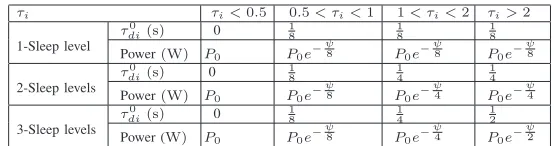
both the case with optimal deactivation latency and the discrete sleep level schemes defined in Table I. In each discrete sleep level, the actual sleep duration of theith

vacation period can be obtained asτsi=τi−(1+η)τdi0,

where the discrete τ_di0 defined in Table I is dependent on the vacation period. Specifically, we consider that

τ_di0 = 0,∀τi <0.5, while discreteτdi0 that corresponds

to other vacation intervals are stated accordingly in Table I for each discrete sleep level. For the case with

θ = 1, ω = 0.5, the parameter τe = 0 in (15) and there exists an optimal deactivation latency for each vacation period. Hence, increasing the mean vacation time leads to a reduction in the average power con-sumption. By increasing the parametersθandωto2and 1, respectively, and consequently the power consumed during the reactivation and deactivation processes, the parameter eτ becomes greater than zero in (15) and

τ⋆

di = 0,∀τi ≤ τe. Hence, in the optimal case, the

BS continues to operate in no-load for all vacation time which is less thanτesince the cost of deactivation and reactivation (increase power during the deactivation and reactivation processes) exceeds the gains from the reduced power consumption due to subcomponent de-activation. This can be seen in Fig. 4 where the average power consumption is equal to P0 for τ¯ ≤0.5 s and

¯

τ ≤ 1 s for the optimal case with θ = 2, ω = 1 and

θ = 3, ω = 1.5, respectively. For the suboptimal case with 3-sleep levels, we observe that the average power consumption initially increases with τ¯to its maximum forθ= 2, ω= 1andθ= 3, ω= 1.5, before decreasing with further increase inτ¯. For the suboptimal case, we observe that the average power consumption could even be higher than the no-load power consumption for some

0 1 2 3 4 5 6 7 8 9 10

Mean vacation time,¯τ_(s)

1 1.2 1.4 1.6 1.8 2 2.2 2.4

P

ow

er

sa

v

in

gs

gai

n

d

u

e

to

τ

⋆,di

P

3-sleep levels,θ_{= 1, ω= 0.5} 2-sleep levels,θ_{= 1}, ω= 0.5 1-sleep level,θ= 1, ω= 0.5 No-load,θ_{= 1}, ω= 0.5 3-sleep levels,θ= 2, ω= 1 2-sleep levels,θ_{= 2, ω= 1} 1-sleep level,θ_{= 2}, ω= 1 No-load,θ= 2, ω= 1

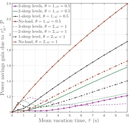
Fig. 5:Power consumption gain due to the use of the optimal deactivation latencyτd⋆against the mean BS vacation timeτ¯.

mean BS vacation time.

In Fig. 5, we plot the power savings gain P due to the use of the optimal deactivation latency against the mean BS vacation timeτ¯. The power savings gainP is obtained as a ratio of the average power consumption due to the use of the sleep levels defined in Table I to the average power consumption based on the selection of the optimal deactivation latency. We benchmark the result with the case with no sleeping, i.e., the BS retains the no-load power consumption during the vacation period. It can be observed that the selection of the optimal deactivation latency always results in power savings gain since P >1,∀τ¯.

V. CONCLUSIONS

In this paper, we have addressed the most energy-efficient BS subcomponent deactivation latency while considering that the BS no-load intervals are known in advance by obtaining a closed-form expression of the deactivation latency that minimizes the average BS power consumption. Our analytical insights have revealed that significant power saving can be achieved by selecting the optimal deactivation latency. In ad-dition, further savings can be achieved by addressing the high power consumption during the subcomponent deactivation and reactivation phases.

ACKNOWLEDGEMENT

TABLE I: Discrete Sleep level

τi τi<0.5 0.5< τi<1 1< τi<2 τi>2

1-Sleep level

τ0

di(s) 0

1 8

1 8

1 8

Power(W) P0 P0e−

ψ

8 _P0e−

ψ

8 _P0e−

ψ

8

2-Sleep levels

τ0

di(s) 0

1 8

1 4

1 4

Power(W) P0 P0e−

ψ

8 _P0e−

ψ

4 _P0e−

ψ

4

3-Sleep levels

τ0

di(s) 0

1 8

1 4

1 2

Power (W) P0 P0e−

ψ

8 _P0e−ψ4 _P0e−ψ2

REFERENCES

[1] Nokia Siemens Networks, ETSI RRS05-024, 2011.

[2] O. Arnold et al., “Power consumption modeling of different base station types in heterogeneous cellular networks,” inProc.

Future Network and Mobile Summit, Florence, Italy, Jun. 2010.

[3] G. Auer et al., “How much energy is needed to run a wireless network?”IEEE Wireless Commun. Mag., vol. 18, no. 5, pp. 40–49, Oct. 2011.

[4] B. Debaillie, C. Desset, and F. Louagie, “A flexible and future-proof power model for cellular base stations,” inIEEE

Vehicular Technology Conference (VTC Spring), 2015.

[5] IMEC, “Power model for today’s and future base stations,” [On-line]. Available: http://www.imec.be/powermodel [Accessed:22 - Feb - 2018].

[6] B. H. Stark, G. D. Szarka, and E. D. Rooke, “Start-up circuit with low minimum operating power for microwatt energy harvesters,”IET Circuits, Devices Systems, vol. 5, no. 4, pp. 267–274, Jul 2011.

[7] L. Wang et al., “Small cell switch policy: A consideration of start-up energy cost,” inIEEE/CIC International Conference on

Communications in China (ICCC), Oct 2014, pp. 231–235.

[8] A. Mohamed et al., “Control-data separation architecture for cellular radio access networks: A survey and outlook,”IEEE

Communications Surveys & Tutorials, vol. 18, no. 1, pp. 446–

465, Firstquarter 2015.

[9] A. Mohamed, O. Onireti, M. A. Imran, A. Imran, and R. Tafa-zolli, “Correlation-based Adaptive Pilot Pattern in Control/Data Separation Architecture,” inIEEE International Conference on

Communications (ICC), Jun 2015.

[10] 3GPP, ”TR 38.913: Study on Scenarios and Requirements for Next Generation Access Technologies”. Tech. Rep., Release 14 Version 0.4.0. June 2016.

[11] P. Lahdekorpi, M. Hronec, P. Jolma, and J. Moilanen, “Energy efficiency of 5G mobile networks with base station sleep modes,” inIEEE Conference on Standards for Communications

and Networking (CSCN), Sept 2017, pp. 163–168.

[12] O. Onireti, A. Mohamed, H. Pervaiz, and M. Imran, “Analytical approach to base station sleep mode power consumption and sleep depth,” inIEEE International Symposium on Personal,

Indoor, and Mobile Radio Communications (PIMRC), Oct.

[13] D. Ferling et al., “D4.3: Final report on green radio technolo-gies,” INFSO-ICT-247733 EARTH, Tech. Rep., Jun 2012. [14] 3GPP TS 36.104 V10.2.0 (2011-04); LTE Technical

Specifica-tion (Release 10).