Clustering Multivariate Functional Data with Phase Variation
Juhyun Park1,* and Jeongyoun Ahn2,**
1Department of Mathematics and Statistics, Lancaster University, Lancaster LA1 4YF, U.K.
2Department of Statistics, University of Georgia, Athens, Georgia 30602-1952, U.S.A.
∗email:[email protected] ∗∗email:[email protected]
Summary. When functional data come as multiple curves per subject, characterizing the source of variations is not a trivial problem. The complexity of the problem goes deeper when there is phase variation in addition to amplitude variation. We consider clustering problem with multivariate functional data that have phase variations among the functional variables. We propose a conditional subject-specific warping framework in order to extract relevant features for clustering. Using multivariate growth curves of various parts of the body as a motivating example, we demonstrate the effectiveness of the proposed approach. The found clusters have individuals who show different relative growth patterns among different parts of the body.
Key words: Curve alignment; Functional clustering; Growth curves; Multivariate functional data; Phase variation.
1. Introduction
The rapid development of technology in recording and storing of data makes it possible to collect simultaneous recordings of several longitudinal variables. Often physiological and bio-logical processes are continuously monitored for a number of subjects, resulting in a set of multivariate longitudinal trajec-tories. When the measurements are viewed as realizations of smooth random functions, the field of functional data analy-sis (FDA) provides a wealthy suite of techniques to explore and analyze such types of data. For an overview, we refer to Ramsay and Silverman (2002, 2005) and Ferraty and Vieu (2006). Although FDA is proven useful to deal with data in the form of curves, its extension to multivariate functional data is not yet fully developed and it is an active area of ongoing research. In this work, we focus on the problem of clustering multivariate functional data.
Multivariate functional data can arise in many different settings. The three-dimensional curves from the coordinates of a geometrical object are a good example. Alternatively, we may observe multiple response curves from the same ob-ject sharing the common underlying process. For example, in functional Magnetic Resonance Imaging, simultaneously measured signals from neighboring voxels could be viewed as replicates of brain signals subject to some regional or spatial variability. Different types or techniques of spectroscopy used to study molecules in chemistry rely on the same principle that molecules absorb specific frequencies that are character-istic of their structure. A well-known example comes from a longitudinal growth study, where measurements of various body parts are simultaneously obtained from the same sub-ject. The growth curves have served as a benchmark dataset for functional data, but mostly discussed in the context of one-dimensional curves (e.g., Ramsay and Silverman, 2005).
The particular dataset that we are interested in, the Z¨urich longitudinal growth study database, includes measurements
on six different variables: height, sitting height, leg height, arm length, bihumeral width (shoulder), and biiliac width (pelvis) (Gasser et al., 1984; Sheehy et al., 1999, 2000). Fig-ure 1 shows an example of the growth response curves, in relative velocity, for the first 10 subjects from boys and girls, respectively. Remarkably, the common characteristics are shared by all the variables.
There is no doubt that the growth process of arms is dif-ferent from that of legs, for example. Nevertheless, it may be assumed that there is a common growth process that co-ordinates differential developments of different body parts. Then, it is of great interest to characterize the growth process and to identify groups with different growth patterns. Earlier works were successful in characterizing the growth process in the analysis of single body part measurements, however, the analysis of joint behaviors of growth of various body parts has been scarcely developed. Sheehy et al. (1999) is the ear-lier reference to attempt to analyze the multiple curves si-multaneously, though more in line with classical multivariate analysis.
When an object is represented by multivariate responses, it is important to take into account the dependence between the responses. There are many standard dependence mea-sures for multivariate Euclidean data, often under certain dis-tributional assumptions. However, it is not so obvious how to embed such concepts into functional data as an infinite-dimensional object, with various sources of variation influ-encing the structure of the curves. Multivariate Functional Principal Component Analysis (MPCA) provides a standard tool to capture the variation in a parsimonious way, utilizing the dependence through covariance function, which is suitable to describe a linear dependence between the curves. Never-theless, the notion of dependence can be closely linked to the scientific questions associated with the data and thus the for-mulation requires a careful consideration.
Age
0 2 4 6 8 10 12 14 16 18
Velocity
arms legs pelvis shoulders sith standh
Age
0 2 4 6 8 10 12 14 16 18
Velocity
[image:2.745.56.542.68.270.2]arms legs pelvis shoulders sith standh
Figure 1. Growth curves in relative velocity for a sample of subjects for different body parts. First 10 subjects in the girls (left) and the boys (right).
Going back to the example, the growth data have several unique features that standard functional clustering methods do not take into account (Gasser et al., 1984; Gasser and Kneip, 1995). Firstly, the main information of the growth pro-cess is contained in the speed of growth, that is, the derivatives of the original measurements. Secondly, the main variation of interest in derivatives occurs inphase, rather than in ampli-tude. In fact, amplitude variation could be dominant in size, but considered as a nuisance for comparison of the speed of growth. In addition, due to the natural limit in size for differ-ent body parts, it is more natural to compare the variables on a standardized scale. Thirdly, although the variables could be made comparable, there is no natural scale to combine infor-mation from different sources once standardization is applied. With these considerations in mind, we consider ways to describe the joint patterns of growth that differentiate de-velopmental phases among the subgroups. For example, one might conjecture that on average,
r
legs grow faster than shoulder;r
arm and shoulder tend to grow together;r
nonuniform growth across different body parts is more com-mon compared to uniform growth of all body parts;r
and so on.To express these ideas in statistical terms, we note that a main signal in growth pattern comparisons is related to the ordering of variables with respect to timing of prominent features, that is, the notion of the phasevariation. Phase variation is well understood in the context of one-dimensional curves, though often considered as a nuisance. Our focus is on capturing a relative phase variation across multiple variables to account for dependence, a distinguishing feature of our methodology in contrast with the existing methods dealing with phase vari-ation. As will become clear, our approach offers a complemen-tary and nonstandard view of the growth pattern.
Our main contributions could be summarized as follows. Although the problem of phase and amplitude variation is
well known in general, its implication in multivariate func-tional data analysis has not been well studied yet. Even if we focus on estimation of phase variation and curve alignment, the multivariate version does not exist because it essentially requires to define a proper concept ofmultivariate monotone functionsat its full generality. The first novelty of our article is the very new formulation of the problem of phase varia-tion in multivariate funcvaria-tional data, and its characterizavaria-tion in terms of different parametrization required. As will be seen later, mathematically as well as practically, the multivariate extension is not unique and it requires serious consideration in the context of the problem at hand. Once said, it sounds obvious, but its implication is far greater. We demonstrate the implications in the context of functional clustering. The second novelty is the new clustering method for phase varia-tion only. As many other new developments, many ingredients of the proposed method are borrowed from existing methods. However, amplitude and phase variations are not comparable to each other, and thus direct translation of amplitude method to phase or a naive mixing and matching strategy does not work. With proper considerations of these issues, we develop a new clustering approach applicable to phase variation only. The third novelty is the application itself. As far as we know, the joint analysis of growth phases has not been done before (possibly due to the difficulty in getting such data), and there is no standard methodology available.
This article is organized as follows. Section 2 introduces the framework for phase variation in multivariate functional curves. Section 3 develops a clustering approach based on multivariate phase variation. Section 4 illustrates numerical performance in terms of simulation studies and a real data example.
2. Functional Data and Source of Variation
principal component analysis (PCA) while phase variation is inherently nonlinear and, without proper adjustment, the analysis as well as its interpretation could be misleading.
2.1. Source of Variation in One-Dimensional Functional Curves
Suppose we observe a sample ofncurves on a compact interval
I=[0, T], subject to measurement error. The ith response curve can be represented asYi(t)=Xi(t)+εi(t),whereεi(t) is
the stationary residual process with E[εi(t)]=0, E[ε2i(t)]=σ
2
and Cov(εi(t), εi(s))=0, s=t. Assume thatXiis an element
ofL2(I).
When the curves share common characteristics subject to individual variability, that is, when we assume there exist a common mean μ and a common covariance function , we may further decompose Xi into Xi(t)=μ(t)+Vi(t), where
E[Vi(t)]=0 and Cov(Vi(s), Vi(t))=(s, t).
Often the observed curves exhibit additional variability in the horizontal direction representing delayed or accelerated responses, for which we introduce the time transformation function or warping functionhand its inverseω=h−1 as
Yi(t)=Xi(t)+εi(t), Xi(ωi(t))=μ(t)+Vi(t), (1)
whereωi(orhi)s are monotonically increasing functions from I to I satisfying the boundary conditions ωi(0)=0 and ωi(T)=T. It is common to assume thatωis are continuously
differentiable. Conceptually, we imagine that there is a com-mon underlying process, often characterized by comcom-mon fea-tures or landmarks, so thatωisummarizes the timings of the
onsets of the common features for theith curve.
Most standard approaches developed in the literature to handle this unwieldy problem of phase variation have taken the view that phase variation is a nuisance and can be ac-counted for in a preprocessing step (Gasser and Kneip, 1995; Ramsay and Li, 1998; Wang and Gasser, 1997, 1999; Gervini and Gasser, 2004; James, 2007; Tang and M¨uller, 2008). Re-cent developments attempt to explicitly model the component of phase as the main step of the analysis, although the pri-mary focus is on amplitude in general (Kneip and Ramsay, 2008; Liu and Yang, 2009; Tang and M¨uller, 2009; Slaets et al., 2012; Peng et al., 2014; Hadjipantelis et al., 2015).
As timings can be measured only relatively, there needs fur-ther constraints. For example, if we decide to use a reference curve, sayX1, then
X1(t)=(μ◦h1)(t)+(V1◦h1)(t)=μ˜1(t)+V˜1(t).
Consequently, the timings of the other curves can be expressed as
Xi(t)=(μ◦hi)(t)+(Vi◦hi)(t) =(˜μ1◦˜hi)(t)+( ˜Vi◦h˜i)(t),
where h˜i(t)=h1−1◦hi(t). For standard one-dimensional
curves, this is often expressed as E[ωi(t)]=i(t), where
common features and the ωi(t) measures delays or
acceler-ations relative to the timings of the representative curve at timet.
2.2. Source of Variation in Multivariate Functional Curves
Suppose now that for each subject, there arepcomponents in the response defined on a common intervalI, denoted byX= (X1, . . . , Xp) and there might be some measurement errors. A
general model could be written as
Yi(t)=Xi(t)+εi(t).
In the presence of phase variability, we introduce a vector of warping functions, denoted by hi=(hi1, . . . , hip) with its
inverseω=h−1 to compensate for horizontal variability.
When it comes to multivariate functional data, the issues of phase and amplitude variations still exist but are more dif-ficult to address due to its inherent geometry (Kurtek et al., 2012; Brunel and Park, 2014). Consequently, an extension to multivariate functional curves is not unique and thus needs some careful consideration. In what follows, we list several plausible parametrizations, each of which is based on a differ-ent underlying data-generating mechanism.
2.2.1. Marginal component-wise warping. The marginal warping is a direct component-wise extension of the one-dimensional curve alignment formulation to multivariate case. Here, we assume that each component has its own average re-sponse pattern and phase variation in individual curves vary only relative to the average response time for each component, independent of other components. Then, we would proceed by repeating one-dimensional registration analysisptimes, that is, for each componentr, r=1, . . . , p, the warping functionωc r
satisfies
E[Xir◦ωcir
(t)]=μr(t), (2)
subject to n−1n
i=1ω
c
ir(t)=t forr=1, . . . , p. This strategy
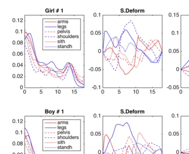
is useful as a preprocessing or the primary interest is the amplitude variation, and also it is the approach taken by most multivariate FDA works. However, as individual ac-celeration/delay is measured relatively within each compo-nent variable, this does not allow us to compare relative de-lays across components. For illustration, an example from the growth data is shown in Figure 2 in the third column.
Figure 2. An example of warping profiles extracted from subject-specific warping (middle) and component-wise warping (right) for the first subject in each group. The left column shows the original growth velocity curves.
ωs
i. Denote theith subject specific average bySi and assume
that
E[Xir◦ωsir
(t)|Xi]=Si(t), (3)
subject top−1p
r=1ω
s
ir(t)=tfor eachi=1, . . . , n. From the
viewpoint of variance decomposition,Si(t) can be regarded as
the conditional mean of the subject-specific random effect. In particular, if the decomposition in (1) were to hold for each component, the subject-specific reference could be identified as μ(t)+E[Vir(t)|Xi], assuming a common trend for all
com-ponents.
Now individual warping profiles (ωs
i) can be compared
be-tween subjects, without reference to the pattern of the pop-ulation average. An example from the growth data is shown in Figure 2 in the second column. This is our model used to extract features of differential growth pattern for each subject for clustering, discussed in Section 3.
2.2.3. Universal warping for all components. In contrast to the previous scenarios, often the registration problem oc-curs in the study of the displacement of an object (e.g., Kurtek et al., 2012; Brunel and Park, 2014) so that the response curves could be identified with respect to some underlying coordinate system. It is then more appropriate to assume a common warping function for all response curves:
E[Xir◦ωi
(t)]=μr(t), r=1, . . . , p ,
subject ton−1n
i=1ωi(t)=t. In this case, the unit of analysis
is the vector of response curves as a whole and the warping function acts as a nuisance parameter in characterizing the variability in the population of the vector of response curves.
3. Multivariate Phase-Cluster Model
Viewing the multiple response curves as a whole unit, we are interested in grouping subjects based on the phase variation differentiating joint growth patterns. When variability in the size or the magnitude of each variable could be of interest, the methodology based on multivariate FPCA could be used (e.g., Jacques and Preda, 2012), and, if necessary, registration methods are combined as a preprocessing (e.g., Ieva et al., 2013). These methods could be efficient but have the same drawbacks as one-dimensional approach when phase variation is of main interest. Sangalli et al. (2010) extend ak-means-like clustering algorithm to three-dimensional curves with phase variation by explicitly specifying a class of (linear) warping functions in the template so that the curves are aligned within each cluster. Brunel and Park (2014) directly focus on general phase variation in so far as estimating the structural mean function but do not address the problem of clustering. In fact, it is a nontrivial problem to find a representation for a cluster center when both variability are present, due to the fact that the functions spaces do not coincide. This is well illustrated in Liu and M¨uller (2004).
can be explained via characterizing the clusters that they set out to find. In the first approach, one can try to find clusters that have different phase patterns (ω) in certain components. The second approach, which is our focus, is to find clusters that have different phase variability across components within an observation.
Figure 2 illustrates extracted features of the first subject in each growth dataset for a comparison. The first column shows the original velocity curves, and the second column shows the curves defined as ˆω(t)−t, called deformation func-tions, from the proposed conditional subject-specific warp-ing in (3). Here, it is expected that the deformation curves have zero mean from the formulation. The crossing patterns in the deformation curves indicate that a measurement vari-able reaches a growth peak earlier than some others and then its growth slows down later. The third column shows the de-formation curves from marginal component-wise warping in (2). Here, the curves are showing how the subject’s growth is delayed or accelerated compared to other subjects in the data, component-wise.
We assume that the population consists of a mixture of Kclusters that have distinct patterns of delays. Our earlier discussion in Section 1 suggests that the dynamic ordering of the warping profiles could be used to define a cluster. How-ever, as the ordering may change continuously over time, this is rather a difficult problem. Instead, we detect the effect of changes in ordering through the relative changes in warping profiles across the component variables. This can be achieved by incorporating the conditional warping as opposed to other types of warping.
3.1. A Phase-Cluster Model
Given the multivariate functional curves, we consider a phase-cluster model represented as follows. Our observation model isYir(t)=Xir(t)+εir(t), i=1, . . . , n;r=1, . . . , p fort∈[0, T]
with
E[Xir(ω
(k)
ir (t))|Xi]=Si(t), for k=1, . . . , K , (4)
subject top−1p r=1ω
(k)
ir (t)=tandω
(k)
ir (0) = 0 andω
(k)
ir (T)= T and K is the number of clusters. Under the subject-specific warping (p−1p
r=1ωir(t)=t), it follows that n−1n
i=1ωir(t)=t for r=1, . . . , p. In particular, if there
is a systematic delay in certain component variable, for example, if shoulder tends to grow later than other body parts on average for subjects in a certain cluster, the corresponding warping function ω for shoulder would tend to lie above the identity line for each individual. Then, on average,n−1n
i=1ωir(t)−ttends to be positive for shoulder.
Motivated by this observation, we define a cluster based on relative delays or deformation function for the ith subject defined byui(t)=ωi(t)−t. It is clear that the relative phase
variations can be translated into the differences in mean of the deformation functions. In addition, the space of the deformation function is better approximated by a linear space and thus alleviates the issues of directly dealing with
Defining clusters may or may not require the information on variability. In order to characterize the cluster in the vector of warping functionsω, we formulate a latent functional mixture model through the deformation functions.
Viewing the deformation functions as an element of L2(I), we assume that u belongs to a Hilbert space H, of
p-dimensional vectors of functions in L2(I). We define a
cluster by its mean function in H, allowing for different variability across the cluster groups. Chiou and Li (2007) proposed a functional K-center clustering for univariate functional data which takes into account variation of the curves through FPCA in defining the cluster center. The same principle can be applied to multivariate functional data, if we replace FPCA by its multivariate version.
To define multivariate functional principal component anal-ysis, we need to define the corresponding norm in the extended function space. For a multivariate function f =(f1, . . . , fp)
withfr2<∞forr=1, . . . , p, define thep-variate norm by f2=p
r=1fr
2. Define the cross-covariance function by
r,s(t, u)=cov(ur(t), us(u)), r, s=1, . . . , p. Denote by (t, u)
the p×p matrix of the cross-covariance function whose (r, s)th element is given by r,s(t, u). Then, the
correspond-ing eigenvalues and eigenfunctions could be defined and the covariance function has the representation as (t, u)=
∞
j=1λjφj(s)φj(t)
T, where λ
js are ordered eigenvalues and φj(t)=(φj1(t), . . . , φjp(t))T are the unit-norm eigenfunctions
satisfying
p
s=1
r,s(t, u)φjs(u)du=λjφjr(t).
Now, we assume that there are Ksubgroups inu. Based on the eigenfunction expansion, we assume that each cluster has its own variability expressed through cluster-dependent eigen-values and eigenfunctions:
u(k)(t)=α(k)(t)+ ∞
j=1
ξ(jk)φ
(k)
j (t), (5)
where ξ(jk) are uncorrelated and E[(ξj(k))2]=λ(k)
j for k=
1, . . . , K.
Putting things together, the phase-cluster model (4) is re-fined to incorporate the additional information on variability for each cluster through (5). Note that within each cluster, amplitude function as well as phase function can vary. In par-ticular, the amplitude functionXcan have its own represen-tation in terms of multivariate FPCA similar to the equa-tion (5).
insists, we can use a monotone parametrization by assuming that dtd logωcan be expressed by the basis function expansion. Here, we keep the additive structure for simplicity as this pro-vides a good approximation to describe the main variability in phase.
3.3. Estimation of Functional Phase-Cluster Model
Although our formulation resembles a standard mixture model, due to identifiability constraints for the latent warping functions, simultaneous estimation of this type of model is not straightforward. On the other hand, the problem is formulated in such a way that estimation of the latent warping functions is not directly related to how they are clustered. In fact, we consider estimation of the warping profiles as the step for fea-ture extraction in clustering multivariate functional curves. Thus, we propose the following two-stage algorithm and give some details in the following.
(i) [Feature extraction by conditional warping] For each subject i, i=1, . . . , n, estimate ωi by subject-specific
warping and obtain deformation function ui(t)= ωi(t)−t.
(ii) [Functional clustering] Apply multivariate functional clustering tou.
3.3.1. Feature extraction by conditional warping. The subject-specific warping amounts to registration of multiple response curves for each subject. Let = {ω:I→I, ω≥ 0, ω(0)=0, ω(T)=T, ωis a diffeomorphism} be the set of warping functions. Fori=1, . . . , n,
(Si,ωi)=arg infS∈L2(I)inf(γ1,...,γp):γr∈
p
r=1
d(Xir◦γir, S).
This problem falls into the general problem of curve alignment for one-dimensional curves, a well-studied area in FDA. Most standard algorithms that treat phase variation as a nuisance are applicable to our case (Gasser and Kneip, 1995; Wang and Gasser, 1997; Ramsay and Li, 1998; Wang and Gasser, 1999; Gervini and Gasser, 2004; Liu and M¨uller, 2004; James, 2007; Tang and M¨uller, 2008; Tucker et al., 2013).
The main difficulty in directly solving this optimization problem is that the reference function S is also unknown so that some form of iteration would be necessary. In ad-dition, the γ is an infinite-dimensional object that should satisfy monotonicity constraints. Different strategies in the choice of the metric d(·,·), the parametrization ofγ∈ , the scheme of updating the reference S, as well as the optimiza-tion algorithm itself lead to different methods. One of the original methods known as landmark registration (Gasser and Kneip, 1995) exploits the fact that features that could iden-tify S are available or could be well estimated using appro-priate smoothing techniques for estimating derivatives. The standard monotone registration method in Ramsay and Sil-verman (2005) uses an explicit monotone parametrization with spline functions and solves iteratively a nonlinear least squares problem. Most methods developed an algorithm based on the standard L2 distance as d(X1, X2)= X1−X22 for
X1, X2∈L2(I) whereas Tucker et al. (2013) based their
al-gorithm on Fisher–Rao metric that compares a normalized derivative function defined as
qX(t)=X˙(t)
|X˙(t)| ·(|X˙(t)| =0),
and dFR(X1, X2)= q1−q2. This formalizes the intuition
that curves are better aligned based on the features in the derivatives. They developed an efficient algorithm based on dynamic programming. Comparison of different registration methods is beyond the scope of the article.
We used the registration method based on the Fisher–Rao metric (Tucker et al., 2013) in our analysis. It is algorithmi-cally efficient and is known to be one of the most successful methods for registration. In our simulation studies, we eval-uate the effectiveness of the registration method and its im-pact on clustering in comparison to the monotone registration method (Ramsay and Silverman, 2005) as a standard refer-ence.
3.3.2. Estimation of functional clusters in deformation function. It turns out that the computation of multivariate FPCA can be simplified for the warping functions. We first define an extended curve as the concatenation of the multi-ple curves over the extended period of time. For each curve ur(t), r=1, . . . , p, ur(0)=ur(T)=0. Let U(t), t∈[0, pT] be
the concatenation of the curves (u1, . . . , up) defined as
U(t)=ur(t), for t∈[(r−1)T, rT].
Denote the mean function byαand the covariance function by (t, u)=Cov(U(t), U(u)). Then,Ucan be identified as a ran-dom process inL2([0, pT]). In terms of procedural definition,
the multivariate FPCA is equivalent to a univariate FPCA with these extended curves. Normally, the one-dimensional view requires additional continuity assumption at end points of each curve, which in general is not always satisfied by mul-tivariate functions. However, viewing the warping function as a diffeomorphism with boundary conditions imposed on implies thatur(0)=ur(T)=0 and thus preserves continuity
in concatenation. Although not required, further smoothness condition could be considered at the boundaries. Now, we re-formulate the clustering problem with the extended curves of the deformation functions as follows. For the population of thekth cluster, we assume that
U(k)(t)=α(k)(t)+
∞
j=1
ξj(k)φ(jk)(t).
Another issue with multivariate functional principal com-ponent analysis is the comparability of the measure of variability across the variables, say Xr, r=1, . . . , p. Chiou
fect the performance being the success of the estimation of the warping profiles and the success of functional clustering method on the curves. In this section, we use simulated data to investigate relative performances of each component, with a standard implementation as a reference. For warping function estimation, the registration method by the Fisher–Rao metric is compared with the standard monotone registration method (Ramsay and Silverman, 2005). For clustering, Chiou and Li (2007)’s functional clustering with concatenated deformation function is compared with high-dimensional curve clustering method implemented in CCToolbox by Gaffney (2004).
As for the settings, we use total six different settings. Among those two are “null” settings for which the signals in data are not necessarily what the proposed method sets out to find. In one of the null settings, the two clusters are different only in their amplitude patterns, for which usual (multivariate) functional clustering approaches would target at. The other null setting is based on the marginal component warping model discussed in Section 2. These two settings are to illustrate that the proposed approach sets out to solve fun-damentally different scientific problems than existing meth-ods to begin with, thus for the null settings we expect to see random assignments in clustering with our approach.
The other four settings are designed to see not only whether the proposed approach works as intended but also which warping method and clustering method works best under var-ious scenarios. As the warping profiles are latent and the am-plitude information is a nuisance for clustering, we consider four distinct scenarios to evaluate the method of extracting phase variation in the presence of amplitude dilution as well as phase variation. The level of dilution is introduced by varying the covariance structure for phase functions in each cluster.
Each observation, belonging to one of the two clusters of sizen=25 each, is a set of four curves (p=4) that are anal-ogous to the different body parts in the growth data example. All curves are defined on the time range−3≤t≤3 and gen-erated asy(t)=S(h(t)), whereS(t) represents the amplitude pattern andh(t) for phase variation. The amplitude of therth component curve in an individual,Sr(t),r=1, . . . ,4 is one of
the following:
S1r(t)=Z1rexp{−.05(t−2)2} +Z2rexp{−10(t+1)2}/6,
S2r(t)=Z1rexp{−.05(t−2)2} +Z2rexp{−10(t+1)4}/6,
whereZkrareN(1, .22),k=1,2,r=1, . . . ,4.
The phase functionhr(t), r=1, . . . , p is constructed based
on a functional PCA model. For scenarios 1-5, let a= (−3,−1,1,3)+Np(0, .52Ip). The mean functions of hr(t), r=1, . . . ,4, are either not crossed
mu r(t)=
6 exp{ar(t+3)/6} −1 ear−1 −3,
+I(t >0) 3 exp{−ar(t+3)/6} −1 ear−1
.
As for the covariance structures ofhr(t), we consider three
cases: (i) φ1
1(t)=0, φ12(t)=0, that is, identity, (ii) φ21(t)=
sin(πt/3)√3, φ2
2(t)=cos(πt/2)/
√
3, (iii) φ3
1(t)= {cos(πt/3)+
1}/3,φ3
2(t)=sin(πt/3)/
√ 3. Then, we set hj,u
r (t)=m u
r(t)+ξ1φ
j
1(t)+ξ2φ
j
2(t)+(t) for
crossed warping and hj,c
r (t)=mcr(t)+ξ1φ
j
1(t)+ξ2φ
j
2(t)+(t)
for uncrossed warping, whereξk∼N(0, θk2),θ1=1 andθ2=.5
and(t) are white noise with variance 0.032.
The six scenarios are introduced below. The first four sce-narios have different mean warping structures within an ob-servation, for which the proposed method aims for:
r
Scenario 1: both clusters have identical amplitude patterns and the common covariance structure for phase variation, S1r(h1r,u(t)) versusS1r(h1r,c(t)). That is, the two clusters arethe same except the crossing pattern of the mean warping functions.
r
Scenario 2: both clusters have identical amplitude patterns, but have different covariance structure as well as mean for phase variation,S1r(h2r,u(t)) versusS1r(h3r,c(t)).r
Scenario 3: clusters have different amplitude patterns, and different mean but identical covariance structure for phase variation,S1r(h3r,u(t)) versusS2r(h3r,c(t)).r
Scenario 4: clusters have different amplitude patterns, and have different covariance structure for phase variation, S2r(h2r,u(t)) versusS1r(h3r,c(t)).r
Scenario 5: (null case) clusters have different amplitude pat-terns, but have identical phase variation.S2r(h2r,u(t)) versus S1r(h2r,u(t)).r
Scenario 6: (a component-wise warping model) letbbe an equal-sized grid ofn=25 on [−3,3] with added Gaussian noise with variance 0.05. Then, ˜ais the randomly permuted version ofbdifferently for each component and each clus-ter. For therth component curve,r=1, ...,4, thejth obser-vation,j=1, ..., nis Yj(t)=S1j(h1,u
j (t)) for Cluster 1 and Yj(t)=S2j(h
1,u
j (t)) for Cluster 2, whereh
1,h
j (t)=muj(t)
ex-cept thatar, r=1, . . . ,4 is replaced with ˜aj, j=1, . . . , n.
For a numerical summary for comparison of the clustering outcomes, we use the Adjusted Rand Index (ARI) score pro-posed by Rand (1971) and Hubert and Arabie (1985). The index is essentially the proportion of the agreements between two partitions. Its value is always between −1 and 1, with −1 corresponding to the perfect disagreement and 1 to the perfect agreement. The value of zero can be achieved between two purely random partitions.
Table 1
Mean warping errors and mean clustering accuracies, measured in adjusted Rand Index, for two choices of warping
methods and two choices of clustering methods
Chiou CCToolbox
Scenario Warping MSE(ˆh) ARI2 ARIK ARI2 ARIK
F–R 0.0864 1.0000 0.9676 0.9984 0.8732 1
Ramsay 0.0981 0.9888 0.7422 0.9936 0.8782
F–R 0.2013 0.9231 0.7960 0.9400 0.8388 2
Ramsay 0.2881 0.4781 0.4053 0.6424 0.4743
F–R 0.1768 0.7846 0.6709 0.8546 0.7150 3
Ramsay 0.2568 0.2442 0.2627 0.4614 0.3715
F–R 0.2130 0.9225 0.8095 0.9228 0.8206 4
Ramsay 0.3064 0.3289 0.2808 0.4489 0.3526
F–R 0.2632 −0.0010 −0.0039 0.0001 −0.0015 5
Ramsay 0.3644 0.0197 0.0146 0.0203 0.0158
F–R N/A 0.0013 0.0115 0.0031 0.0041 6
Ramsay N/A −0.0026 −0.0027 −0.0035 −0.0049
K. The CH index is analogous to the F-ratio statistic, that is, the ratio of between cluster variation and within cluster variation, each adjusted for respective degrees of freedom.
Table 1 summarizes the simulation results based on 50 rep-etitions. First, we report the mean squared error of the esti-mated warping function computed as
MSE(ˆh)=(np)−1
n
i=1
p
r=1
I
(ˆhir(t)−hir(t))2dt ,
to compare the accuracy in estimation of warping profiles. Note that in Scenario 6, we do not report MSE, since it is not relevant to the considered model. Also, we report ARI when we fix K=2 (ARI2) and also when we let CH index choose
K(ARIK).
The findings can be summarized as follows:
r
F–R warping is more accurate than Ramsay’s method, in terms of MSE, which affects the subsequent clustering re-sults.r
Under the null settings, that is, Scenarios 5 and 6, the pro-posed method does not yield a meaningful clustering, which is desirable.r
Chiou’s clustering is better in Scenario 1 while CCTool-box is better in Scenario 3, especially in ARI2. With F–Rwarping, the difference between clustering methods is not substantial in Scenarios 2 and 4.
r
Performance patterns are similar whenKis fixed and when Kis adaptively chosen, the latter generally yields a bit lower ARI.4.2. An Application to Multivariate Growth Curves
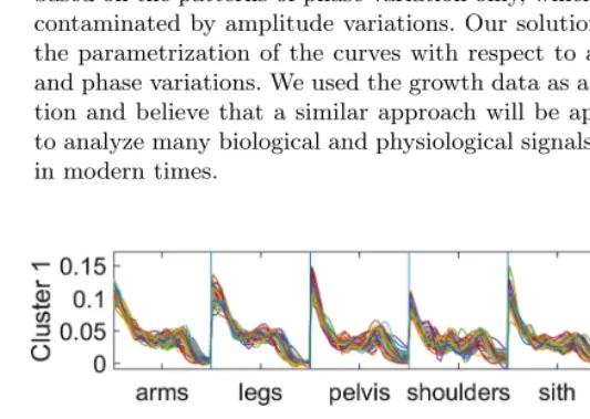
[image:8.745.44.290.118.305.2]We analyze the growth data, introduced in Section 1 with a goal to identify subgroups that have different comparative ac-celeration/delay patterns among different body measurement growths. We standardize the original curves and consider the
Figure 3. Clusters found in the girls. Deformation curves are shown. Cluster mean curves show differences in relative growths among legs, shoulders, and sitting heights.
velocity as the response curves. In any clustering analysis, verifying whether found clusters are “meaningful” is not a straightforward problem. In this work, in order to verify the clusters, we randomly split data into two groups, say A and B, run the clustering in A, and using the cluster centers in A, we assign the individuals in B. Then, we run the cluster-ing algorithm in B and compare the two cluster assignments in B in terms of ARI. We repeated this 50 times. As for the number of clusters, we chooseK=2, which yields the lowest ARIs. For the girls, mean ARIs with Chiou and CCToolbox are, respectively, 0.6205 (0.1745) and 0.2024 (0.2344) with standard deviation inside the parentheses. For the boys, the ARIs are 0.0859 (0.1707) and 0.0469 (0.0801), which indicates no meaningful clusters.
Results show that for girls, there are two clusters that show clearly different patterns in the warping functions. Main dis-tinction is in the relative delay pattern in leg length, shoul-ders, and sitting, as shown in Figure 3. The girls in the first cluster (n=60) share the pattern that legs grow rapidly at the earlier ages while the growth spurt of legs of the girls in the second cluster (n=42) relatively constant and longer lasting.
It is of interest to see how the above cluster solution is com-pared with the clustering with original velocity curves or the warped velocity curves that contain (supposedly) only am-plitude variation left after warping. We also compare results based on the component warping approach. Table 2 shows the disagreements among the cluster solutions based on different types of curves. As a reference, Figure 4 shows the found clus-ters with original curves. It is clear that the usual clustering with multivariate functional curves has a fundamentally dif-ferent goal than our problem presented here.
5. Discussion
33 27 33 27 33 27 39 21 60 Phase
21 21 21 21 21 21 31 11 42
Total 54 48 54 48 55 47 70 32 102
Boys Original Amplitude C. Amplitude C. Phase Total
31 8 27 12 28 11 18 21 39
Phase
43 17 31 29 35 25 26 34 60
Total 74 25 58 41 63 36 44 55 99
rather limited and phase variation is rarely the focus of the main analysis. Notably, many statistical procedures developed for FDA are inherently linear, relying on the linear represen-tation of an object in a Euclidean space, while phase variation is an exception. Recent interests in geometrical approaches in data analysis will become more relevant (e.g., Kurtek et al., 2012), though its exploration in the context of FDA is still in its infancy. We demonstrated the importance and utility of proper consideration of the problem in the context of clus-tering multivariate functional data. In contrast to standard clustering problems, our targets are implicitly defined groups based on the patterns of phase variation only, which could be contaminated by amplitude variations. Our solution exploits the parametrization of the curves with respect to amplitude and phase variations. We used the growth data as an illustra-tion and believe that a similar approach will be appropriate to analyze many biological and physiological signals collected in modern times.
Figure 4. Clusters found in the girls with original velocity curves. Mean curves show that the differences between the two clusters are mostly in the shoulder growths.
Acknowledgements
We thank the Editor, Associated Editor, and two anonymous referees for their careful reading and useful suggestions that lead to many improvements in the article.
References
Brunel, N. and Park, J. (2014). Removing phase variability to ex-tract a mean shape for juggling trajectories.Electronic Jour-nal of Statistics8, 1848–1855.
Calinski, T. and Harabasz, J. (1974). A dendrite method for cluster analysis.Communications in Statistics3, 1–27.
Chiou, J.-M., Chen, Y.-T., and Yang, Y.-F. (2014). Multivariate functional principal component analysis: A normalization approach.Statistica Sinica24, 1571–1596.
Chiou, J.-M. and Li, P.-L. (2007). Functional clustering and iden-tifying substructures of longitudinal data. Journal of the Royal Statistical Society, Series B69, 679–699.
Ferraty, F. and Vieu, P. (2006). Nonparametric Functional Data Analysis. Springer Series in Statistics. Theory and Practice. New York: Springer.
Gaffney, S. (2004).Probabilistic Curve-Aligned Clustering and Pre-diction with Mixture Models. PhD thesis, University of Cal-ifornia, Irvine.
Gasser, T. and Kneip, A. (1995). Searching for structure in curve sample.Journal of the American Statistical Association90, 1179–1188.
Gasser, T., M¨uller, H. G., K¨ohler, W., Molinari, L., and Prader, A. (1984). Nonparametric regression analysis of growth curves.
Annals of Statistics12, 210–229.
Gervini, D. and Gasser, T. (2004). Self-modeling warping functions.
Journal of the Royal Statistical Society, Series B66, 959– 971.
Hadjipantelis, P. Z., Aston, J., M¨uller, H. G., and Evans, J. P. (2015). Unifying amplitude and phase analysis: A composi-tional data approach to funccomposi-tional multivariate mixed-effects modeling of Mandarin Chinese. Journal of the American Statistical Association110, 545–559.
Hubert, L. and Arabie, P. (1985). Comparing partitions.Journal of Classification2, 193–218.
Ieva, F., Paganoni, A. M., Pigoli, D., and Vitelli, V. (2013). Mul-tivariate functional clustering for the morphological analysis of electrocardiograph curves.Journal of the Royal Statistical Society Series C62, 401–418.
Jacques, J. and Preda, C. (2012). Model-based clustering for multi-variate functional data.Computational Statistics and Data Analysis1, 1–24.
James, G. (2007). Curve alignment by moments.Annals of Applied Statistics1, 480–501.
Kneip, A. and Ramsay, J. O. (2008). Combining registration and fitting for functional models.Journal of the American Sta-tistical Association103, 1155–1165.
Kurtek, S., Srivastava, A., Klassen, E., and Ding, Z. (2012). Statis-tical modeling of curves using shapes and related features.
[image:9.745.64.331.499.688.2]Liu, X. and M¨uller, H. G. (2004). Functional convex averaging and synchronization for time-warped random curves.Journal of the American Statistical Association99, 687–699.
Liu, X. and Yang, C. (2009). Simultaneous curve registration and clustering for functional data.Computational Statistics and Data Analysis53, 1361–1376.
Peng, J., Paul, D., and M¨uller, H. G. (2014). Time-warped growth processes, with applications to the modeling of boom-bust cycles in house prices.Annals of Applied Statistics8, 1561– 1582.
Ramsay, J. O. and Li, X. (1998). Curve registration.Journal of the Royal Statistical Society, Series B60, 351–363.
Ramsay, J. O. and Silverman, B. W. (2002). Applied Functional Data Analysis: Methods and Case Studies. Springer Series in Statistics. New York: Springer-Verlag.
Ramsay, J. O. and Silverman, B. W. (2005).Functional Data Anal-ysis. Springer Series in Statistics, second edition. New York: Springer.
Rand, W. M. (1971). Objective criteria for the evaluation of clus-tering methods.Journal of the American Statistical Associ-ation66, 846–850.
Sangalli, L., Secchi, P., Vantini, S., and Vitelli, V. (2010). K-means alignment for curve clustering.Computational Statistics and Data Analysis54, 1219–1233.
Sheehy, A., Gasser, T., Molinari, L., and Largo, R. H. (1999). An analysis of variance of the pubertal and mid-growth spurts for length and width.Annals of Human Biology26, 309–331. Sheehy, A., Gasser, T., Molinari, L., and Largo, R. H. (2000). Con-tribution of growth phases to adult size.Annals of Human Biology27, 281–298.
Slaets, L., Claeskens, G., and Hubert, M. (2012). Phase and amplitude-based clustering for functional data. Computa-tional Statistics and Data Analysis56, 2360–2374. Tang, R. and M¨uller, H. G. (2008). Pairwise curve synchronization
for functional data.Biometrika95, 875–889.
Tang, R. and M¨uller, H. G. (2009). Time-synchronized clustering of gene expression trajectories.Biostatistics10, 32–45. Tucker, J. D., Wu, W., and Srivastava, A. (2013). Generative
mod-els for functional data using phase and amplitude separation.
Computational Statistics and Data Analysis61, 50–66. Wang, K. and Gasser, T. (1997). Alignment of curves by dynamic
time warping.Annals of Statistics25, 1251–1276.
Wang, K. and Gasser, T. (1999). Synchronizing sample curves non-parametrically.Annals of Statistics27, 439–460.