Three essays on the predictive content and predictability of the nominal exchange rates in a changing world

Three Essays on the Predictive Content and Predictability of

the Nominal Exchange Rates in a Changing World

Panteleimon Promponas

This thesis is submitted in partial fulfilment of the requirements for the degree of Doctor of Philosophy at the Department of Economics, Lancaster University.

ii

Declaration

I hereby declare that this thesis has been composed solely by myself and that it has not been submitted, in whole or in part, for any other degree.

Panteleimon Promponas

iii

To my family

iv

Acknowledgments

I would like to express my deep and sincere gratitude to my supervisors, Prof David Peel and Prof Mike Tsionas, for their excellent guidance and support throughout this journey. Also, I would like to thank Dr Efthymios Pavlidis for his constructive comments and encouragement.

I am also grateful to my parents and brother for their unwavering support, and to my beloved Eleni, for her encouragement, understanding and patience. Special thanks to my Greek friends for making me laugh at difficult moments.

v

Table of Contents

1. Introduction ... 1

Introduction ... 1

2. Forecasting the Taylor rule fundamentals in a changing world: The case of the U.S. and the U.K. ... 4

2.1 Introduction ... 4

2.2 Monetary policy and structural breaks of U.S. and U.K. ... 7

2.2.1 Bai and Perron tests for multiple structural changes in the Taylor rule of the U.S. and the U.K. ... 12

2.3 Motivation and TVP-BVAR forecasting model ... 17

2.4 Data and real-time forecasting exercise ... 21

2.4.1 Forecast implementation and evaluation ... 23

2.5 Empirical results ... 25

2.6 Conclusions ... 29

3. Forecasting the nominal exchange rate movements in a time-varying enviroment: The case of the U.S. and the U.K. ... 31

3.1 Introduction ... 31

3.2 Exchange rate models and predictors ... 34

3.3 Linear and non-linear models ... 43

3.4 Models, data, and forecasts ... 53

3.5 Empirical results and discussion ... 56

3.6 Conclusions ... 65

4. Exchange rates and foreign policy crises. An in-sample and out-of-sample analysis ... 68

4.1 Introduction ... 68

4.2 Literature review ... 69

4.3 Data structure and descriptive statistics ... 74

4.4 Empirical results ... 79

4.4.1 In-sample results ... 79

4.4.2 Out-of-sample results ... 83

5. Conclusions ... 87

Conclusions ... 87

6. Appendix A ... 90

Bai and Perron (1998, 2003) test ... 90

vi

7. Appendix B... 95

BVAR(p) model ... 95

Homoscedastic TVP-BVAR(p) model ... 96

Heteroscedastic TVP- BVAR(p) model ... 100

Dynamic Model Averaging and Selection ... 102

DSGE model’s micro-foundations ... 105

8. Appendix C ... 116

9. Bibliography ... 122

List of Figures

Figure 2.2: Inflation rate, short-term nominal interest rate, and output gap (HP filtered) ... 13

Figure 3.1 Time-varying posterior probability of inclusion of predictors for the 1-quarter-ahead horizon ... 64

Figure 4.1: Graph plotting some of the major historic violent and non-violent FPCs, along with the nominal USD/GBP exchange rate over the period 1971‒2013 ... 77

vii

List of Tables

Table 2.1: Bai and Perron (1998) multiple breakpoint tests of the U.S. policy rule ... 14

Table 2.2: Bai and Perron (1998) multiple breakpoint tests of the U.K. policy rule .. 16

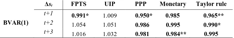
Table 2.3: Relative RMSFE of candidate models for h = 1, 2, 3 and 4 periods ahead 25 Table 2.4: Relative MAFE of candidate models for h = 1, 2, 3 and 4 periods ahead . 26 Table 2.5: Relative RMSFE of candidate models for h = 1, 2, 3 and 4 periods ahead 27 Table 2.6: Relative MAFE of candidate models for h = 1, 2, 3 and 4 periods ahead . 28 Table 3.1: Relative RMSFE of the BVAR(1) models vs. the RW model for h = 1-, 2- and 3-quarters ahead ... 57

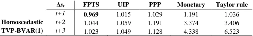
Table 3.2: Relative RMSFE of the homoscedastic TVP- BVAR(1) models vs. the RW model for h = 1-, 2- and 3-quarters ahead ... 58

Table 3.3: Relative RMSFE of the heteroscedastic TVP- BVAR(1) models vs. the RW model for h = 1-, 2- and 3-quarters ahead ... 59

Table 3.4: Relative RMSFE of the homoscedastic TVP- BVAR(1) models vs. the RW model for h = 1-, 2- and 3-quarters ahead ... 61

Table 3.5: Relative RMSFE of the heteroscedastic TVP- BVAR(1) models vs. the RW model for h = 1-, 2- and 3-quarters ahead ... 61

Table 3.6: Relative RMSFE of Bayesian DMA-DMS models vs. the RW model for h = 1-, 2- and 3-quarters ahead ... 62

Table 3.7: Relative RMSFE of the DSGE model vs. the RW model for h = 1-, 2- and 3-quarters ahead ... 65

Table 4.1: Foreign Policy Crises descriptive statistics ... 78

Table 4.2: Fama-based models’ OLS results ... 81

Table 4.3: PPP-based models’ OLS results... 81

Table 4.4: Monetary-based models’ OLS results ... 82

Table 4.5: Taylor-rule models’ OLS results ... 82

Table 4.6: Fundamentals-based out-of-sample results ... 85

Table A.1: Clark and West (2006) test statistics of Table 2.3 ... 93

Table A.2: Clark and West (2006) test statistics of Table 2.5 ... 94

Table B.1: Prior selection and estimated posterior means of the DSGE parameters 113 Table B.2: Data transformation for the DMA and DMS analysis... 114

Table B.3: Clark and West (2006) test statistics of Tables 3.1 ‒ 3.7 ... 115

viii

Abstract

This thesis examines the predictive power and the predictability of the nominal USD/GBP exchange rate changes in a world with structural instabilities. In Chapter 2 we mainly focus on the predictive content of the exchange rates in an attempt to forecast the Taylor rule fundamentals, such as the output gap, the inflation rate and the real exchange rate of the U.S. and the U.K. We employ time-varying econometric techniques, taking into account possible non-linearities and time-variations of the Taylor rule relationships, while we also use Bayesian methods and real-time (vintage) data for the variables that suffer from consecutive revisions. Chapter 3 reviews the well-known ‘Meese and Rogoff’ puzzle which describes the inability of the macroeconomic

1

Introduction

In the world of today, currency is one of the principal driving forces of a national economy and is exchanged for trading purposes. People traveling around the world may need to hold foreign currency for personal transactions, while international firms and governments demand foreign currency for importing products or buying services from abroad. Hence, the exchange rate of two currencies plays a crucial role in consummating a transaction at an international level, as well as bridging the economic and financial relationship of different countries or parties around the world.

Given the importance of the foreign exchange rates, researchers are very keen to explore their behaviour, dynamics, predictive content and relationship with

macroeconomic variables such as theGDP, the inflation rate, the interest rate and the

money supply. Engel and West (2005) find that exchange rates Granger-cause the Taylor rule fundamentals, concluding that exchange rates are likely to be more useful in forecasting the fundamentals than the opposite. This scenario was examined using an in-sample framework, revised data and assuming structural stability of the Taylor rule relationships. In Chapter 2, we novelly extend this idea by investigating the out-of-sample predictive content of the exchange rates in forecasting the Taylor rule fundamentals (output gap, inflation and real exchange rate) of the U.S. and the U.K. We employ time-varying econometric techniques, taking into account the possible non-linearities and time-variations of the Taylor rule relationships, while we also use real-time (vintage) data for the variables that suffer from consecutive revisions. Finally, we employ Bayesian econometric methods, which have become increasingly interesting, to draw a priori more predictive power from the exchange rates than the rest predictors. The interest in this exercise is whether Engel and West’s (2005) findings are robust under the different data structure, environment and methods that we examine.

2

puzzle’, due to the seminal and influential empirical works of Meese and Rogoff (1983a, 1983b). Apart from the ‘disconnection’ issue described in their research papers, they also pinpoint the fact that a ‘naïve’ a-theoretical random walk model is more capable of forecasting the exchange rate movements, than any other more complex and sophisticated economic model, especially at short horizons. Hence, this puzzle has led many researchers to develop several econometric techniques, theoretical and empirical models in an attempt to overturn these findings and generate better forecasts than the benchmark random walk model.

In Chapter 3, we revisit the aforementioned puzzle by conducting a real-time exchange rate (USD/GBP) forecasting race between theoretical and empirical models proposed by the existing literature and the driftless random walk model which seems to be the toughest benchmark model. We include a wide range of models based on traditional macroeconomic predictors as well as a structural DSGE model which describes and mimics the behaviour of the economies. We pay special attention to the time-variations and the unstable relations between the predictors of our models and the exchange rates by employing and comparing the forecasting performance of various homoscedastic and heteroscedastic TVP-Bayesian VAR models. In addition, a Dynamic Model Averaging and Selection developed by Raftery et al. (2010), is included in the race, allowing for a different set of predictors to hold at each time period, and hence, indicating which fundamentals are more relevant in forecasting the exchange rate returns and at which periods. This forecasting race is of particular interest to the reader, as it compares models with different specification, predictors and complexity level, with results indicating which model has the best out-of-sample performance and which predictors are more relevant.

3

categorise them into crises that start, terminate or being under way in each time period. The results of this chapter indicate the usefulness of the foreign policy crises as an additional predictor of the theoretical and empirical exchange rate models.

4

Forecasting the Taylor Rule Fundamentals in a Changing

World: The Case of the U.S. and the U.K.

2.1 Introduction

Since the empirical work of Meese and Rogoff (1983a, 1983b), it has been well known that theoretical exchange rate models based on macroeconomic fundamentals cannot outperform the naïve random walk in out-of-sample accuracy. Forecasting exchange rate changes using the macroeconomic fundamentals as predictors has become an ‘arena’ and debate for many researchers who want to overturn this pessimistic finding.

Engel and West (2005) introduce a key theorem explaining the random walk behaviour of the exchange rates and move to shift the terms of the debate by postulating the question of whether the exchange rates can predict the fundamentals. Using the Taylor rule of two countries, they derive a model within the asset-pricing framework, focusing on the in-sample predictability by conducting Granger-causality tests between the exchange rate changes and the fundamentals. They conclude that the exchange rate changes Granger-cause the macroeconomic fundamentals, such as the relative money supplies, outputs, inflation rates and interest rates, compared to the far weaker causality from the fundamentals to the exchange rates. This finding lead them to underline the fact that the exchange rate changes are likely to be useful in forecasting the future values of the fundamentals. They examine this scenario using the bilateral exchange rates of the U.S. dollar versus the currencies of Canada, France, Germany, Italy, Japan, and the United Kingdom, using revised data for the inflation and the output, while structural

stability in the interest rate reaction functions is also assumed.1

This chapter is mainly motivated from the empirical work of Engel and West (2005) (hereafter EW05), though we take it a step further, building an out-of-sample

1 _{The study of Engel and West (2005) is a remarkable one, testing the predictive content of the exchange}

5

forecasting exercise for the Taylor rule fundamentals (output gap, inflation, and real exchange rate) recognising the need of many institutions, central banks, governments, and practitioners for reliable forecasts of the major macroeconomic variables. We use the Taylor rule introduced by Taylor (1993), and after some modifications introduced by Engel and West (2006), Molotdsova and Papell (2009), and Clarida, Gali and Gertler (1998), we allow (by imposing the appropriate priors) for the exchange rate changes to forecast the fundamentals using a vector autoregressive (VAR) framework, where time-variation in the parameters of the Taylor rule relationships is allowed as well. Existing literature supports the view that interest rate reaction functions suffer from structural changes, non-linearities, asymmetric information and preferences or shifts of the monetary policy behaviour every time the chairmanship of a Central Bank changes (see, e.g. Surico, 2007; Castro, 2011; Nelson, 2000; Dolado et al., 2004). Also, D’Agostino

et al.(2013), Primiceri (2005), and Sarantis (2006) argue that economies in countries

around the world have undergone many structural changes, and models should incorporate mechanisms in order to evolve over time and deliver better forecasts. Therefore, a Bayesian TVP-VAR model, allowing for both intercept and coefficients to change over time, will provide us with the forecasting equations we need for the Taylor

rule fundamentals and also allow us to draw a priorimore predictive power from the

exchange rates than the rest of the predictors.

In this work, we employ vintage (or real-time) data compared to EW05 who use revised data for the output and inflation, since Orphanides (2001) shows that evaluating Taylor rules using ex post revised data leads to different policy reactions than estimating

them with real-time data2. Therefore, he argues that analysis and evaluation of the

monetary policy decisions must be based on information available in real time. Also, Croushore and Stark (2001), Stark and Croushore (2002), and Croushore (2011) present the benefits and forecasting gains that a researcher may have by employing a real-time dataset (such as that developed in the Federal Reserve Bank of Philadelphia with the

cooperation of the University of Richmond).3 All of the aforementioned studies argue

2 _{According to Croushore (2006), ‘vintage’ refers to the date at which the data become publicly available.}

From now on, we call ‘vintage data’ the available observations as announced on a specific date and the collection of those vintages ‘time dataset’. A detailed description of the triangular structure of a real-time dataset can be found in Croushore and Stark (2001).

6

that results from forecasting exercises may be misleading when revised data are used rather than data that were available to the agents at the time they were generating the forecasts. It is striking that Croushore (2011) concludes with the remark that there is no excuse for someone who wants to conduct a forecasting exercise or a policy analysis not to employ real-time data as, nowadays, they are easily accessible and widely

known.4 Hence, we carry out a real-time forecasting exercise using vintage data rather

than an out-of-sample exercise with fully revised data.

A multiple equation vehicle based on real-time information will help us measure how these unstable policy rules affect the rest of the economy by generating 1-, 2-, 3-

and 4-quarters-ahead iterated forecasts for the Taylor rule fundamentals using both

recursive and rolling regressions. We consider the U.S. as the home country and the U.K. as the foreign country. We also include, for comparison purposes, a BVAR and a classical VAR model in the forecasting exercise, while the forecasting performance of the models is compared with that of the driftless random walk model using the relative root mean squared forecast error (RMSFE) and the relative mean absolute forecast error (MAFE) ratios. Clark and West’s (2006, 2007) test of predictive superiority is also used for the significance of the out-of-sample results.

Our main findings show that the TVP-BVAR model, which draws a priori more predictive content from the exchange rates, is able to generate good forecasts for the U.S. output gap, the U.K output gap at longer horizons, the U.K. real exchange rate at the short horizon, and the U.K. inflation under the rolling scheme only. To the best of our knowledge, there is no previous study extending EW05’s work in these directions.

The remainder of this chapter is structured as follows. In section 2, we examine the monetary policy of the U.S. and the U.K., with evidence from the literature and our own empirical findings about their structural changes and instabilities. Section 3 elaborates on the specification and the estimation methodology of our TVP-BVAR model, while, in section 4, the real-time data, forecast implementation, and evaluation are discussed. Section 5 summarises the empirical results, and section 6 provides the conclusions.

4 _{Nevertheless, we must mention and encourage the national statistical offices around the world to try}

7

2.2 Monetary policy and structural breaks of U.S. and U.K.

In an attempt to describe the U.S. monetary policy reaction function in an environment in which the debate between discretionary and algebraic-rule policies was taut, and admitting the difficulty in formulating an appropriate algebraic formula that monitors the macroeconomic figures, John Taylor introduced in 1993 an interest rate reaction function known as the ‘Taylor rule’. Hence, according to Taylor (1993), there should

be a balance between discretion and policy rules in the sense that, together, the critical thinking, reasoning, and technical formulas should be the optimal tool for the policymaker. He argues that monetary authority in the U.S. changes the short-term nominal interest rates (Federal fund rates) in response to the deviations in the inflation rate from its target level and real output from its potential level. The reaction function can be written as:

i_t* (_t *)y_tgap _t r, (2.1)

where i_t* is the target for the short-term nominal interest rate, t is the inflation rate,

*

t

 is the target rate of inflation, y_tgap is the output gap (deviation of actual real GDP

from its estimated potential level), and r″ is the equilibrium real interest rate. Taylor

(1993) advocates that the representative Fed policy function might set α = β = 0.5, an

inflation target of 2%, and an equilibrium real interest rate of 2% as well. Hence, the

interest rate should respond with fixed positive weights to the inflation and output gap.5

The above equation can be written as:

i_t*  y_tgap_t, (2.2)

where  r"a*and 1a. When  1 (positive deviation of inflation from its

target level), the literature refers to it as the Taylor-principle and the short-term nominal

interest rate should be increased more than 1:1 with inflation, achieving an increase in the real interest rate.

8

Clarida et al. (1998) and Woodford (2003)consider the possibility that central banks

smoothly adjust their short-term nominal interest rate as:

i_t (1)i_t*i_t1u_t, (2.3)

where [0,1] captures the smoothing rate of the adjustment and ut is assumed to be

an i.i.d. process. With regard to the standard backward-looking version of the Taylor

rule, which is considered in this chapter, one can derive the estimable equation, combining equations (2.2) and (2.3):

i_t __t _yy_tgap i_t1_t, (2.4)

where  (1), y (1) and (1).

The monetary policy rule can also be derived from the solution of an intertemporal optimisation problem in which the central bank minimises a symmetric quadratic loss function with a linear aggregate supply function (Surico, 2007). Castro (2011) mentions that symmetry of the loss function is not the case in the real world. Different weights of positive and negative inflation and output gap may be assigned by the monetary authorities, leading to asymmetric preferences, and therefore, to a non-linear Taylor rule (see, e.g. Nobay and Peel, 2003). Also, in an attempt to interpret Blinder’s (1998) words (when Blinder was describing his experience as Vice Chairman of the Fed), Surico (2007) pinpoints the fact that political pressure may cause the central bank to intervene asymmetrically.

Dolado et al. (2004) construct a model that considers both asymmetries in the preferences of the central bank and non-linearities of the Phillips curve, where the aggregate supply curve is a convex function of the output gap. They also consider the case in which the non-linear Taylor rule gives rise to the sign and size asymmetries.

Sign asymmetry appears when the response to an increase in inflation is larger than the

response to a decrease, although they may have the same magnitude. What they call size

asymmetry is the non-linear relation between the change in the interest rate and the change in the inflation rate. They focus on the periods 1970:M1–1979:M6 and 1983:M1 –2000:M12, which correspond to the chairmanships of the central bankers Arthur

9

results indicate that, prior to 1979, the Fed’s policy could be well described by a linear Taylor rule, and the central bank preferences becoming quadratic in inflation, while after 1983 U.S. interest rate reaction function seems to be described more accurately from a non-linear Taylor rule since it responds more aggressively to the inflation volatility than to the level. They conclude that, during the Volcker–Greenspan period, asymmetric central bank preferences for the inflation appeared with positive deviations of the inflation from the target, which are weighted more than the negative ones.

A slightly different model is that of Surico (2007), who derives the analytical solution of the central bank’s problem, whereby, at the same time, the monetary transmission mechanism is New-Keynesian and asymmetric preferences in both inflation and output gap are allowed. He finds that U.S. monetary policy followed a non-linear Taylor rule during the pre-Volcker period, with the asymmetry being detected in the fact that the Fed assigned less weight to output expansion than output contraction of the same magnitude. However, results for the period after 1982 strongly suggest the symmetric preferences of the central bank. Furthermore, of great importance are the public speeches and interviews of ‘strong’ people who worked for the Fed and U.S. government. Surico (2007) cites a conversation (quoted from Nelson, 2005) between U.S. President Nixon and Arthur Burns (Chairman of the Fed) and some lines

from Nixon’s interview in the Kansas City Star in 1970 (quoted from De Long, 1997).

Nixon argues in the newspaper interview in the Kansas City Star that:‘[the consensus

for Mr. Burns at his swearing-in] is a standing vote of approval, in advance, for lower

interest rates. […] I have very strong views, and I expect to present them to Mr. Burns.

I respect his independence, but I hope he independently will conclude that my views are

the right ones.’

Conversation between Nixon and Burns: ‘I know there’s the myth of the autonomous

Fed... [short laugh] and when you go up for confirmation some Senator may ask you

about your friendship with the President. Appearances are going to be important, so

you can call Ehrlichman (Assistant to President Nixon for Domestic Affairs) to get

messages to me, and he’ll call you.’

10

money growth) and hence probably gaining greater reputation and numbers of voters, at the end of the day.

A different perspective in testing and estimating the monetary policy rule is conducted by Castro (2011), using a logistic smooth transition regression (LSTR) model, which allows for smooth endogenous regime (policy rule) switches, while an LM test is used to draw inferences as to whether the U.S. policy rule follows a linear or an LSTR model. Results show that, during the period 1982:M7–2007:M12, the Fed was targeting an average target of inflation of around 3.5%, while it can almost be characterized by a forward-looking linear Taylor rule since the linearity hypothesis of the forward-looking model is rejected only at 10% significance level against the LSTR model. Regarding the case of U.K., the non-linear STR model is estimated for the period 1992:M10–2007:M12, indicating that the Bank of England (BoE) reacted actively to inflation when the inflation rate was outside the target range of 1.8%–2.4%, whereas once inside it responded only to the output gap. On the other hand, Martin and Milas (2004) study the behaviour of monetary policy in the U.K. before and after 1992 using a forward-looking policy rule adopting an inflation targeting. They find that, in the post-1992 period, monetary authorities followed an asymmetric policy, trying to keep inflation between 1.4% and 2.6%, whereby central bank responded more aggressively when inflation was above this target and more passively to the negative inflation gaps.

A hyperbolic tangent smooth transition regression (HTSTR) model is used by Cukierman and Muscatelli (2008), who estimate the model after breaking down their sample into four periods: 1960:M1–1970:M1, 1970:M2–1979:M3, 1982:M4–1987:M3, and 1987:M4–2005M4, corresponding to the chairmanships of Martin, Burns–Miller, Volcker, and Greenspan, respectively, in the U.S. Fed. During Martin’s period, authors suggest that Fed preferences were more averse to positive than to negative inflation gaps

– what they call inflation-avoidance preferences (IAP). As for the Burns–Miller and

Greenspan periods, although there is no evidence for non-linearity in inflation, the authors find the Fed being more averse to negative than to positive output gaps – what

they call recession-avoidance preferences (RAP). The results for Volcker’s period

11

U.K., the results suggest that the 1979:M3–1990:M3 period is characterised by RAP, while the 1992:M4–2005:M4 period is characterised by IAP.

A three-regime threshold regression model, motivated by Orphanides and Wilcox (2002) and Taylor and Darvadakis (2006), is used in Lamarche and Koustas (2012) to capture possible asymmetries in the Fed’s reactions. Covering the period 1982:M3– 2003:M4 (the Volcker–Greenspan period) and using the expected inflation as threshold, they suggest that the Fed followed a non-linear reaction function, behaving completely differently in the two outer regimes. More specifically, when expected inflation lay within the middle–regime (2.8%–3.9%), it seems that the Fed behaved with policy inaction. However, when expected inflation exceeded the upper threshold, authorities reacted aggressively to cool down the economy, whereas, in the case in which expected inflation appeared below the lower threshold, the policy reaction was to decrease the real interest rates. On the other hand, Taylor and Darvadakis (2006) employ both two- and three-regime models to examine the behaviour of the reaction function of the U.K. for the period 1992:M10–2003:M1. They find that, when the inflation rate exceeded the threshold of 3.1%, a forward-looking Taylor rule was followed by the BoE, with more weight attached to the expected inflation deviations from the target than deviations of the output, however, when inflation was lower than 3.1%, a near random walk process with very small but significant responses to the output gap characterised the interest-rate-setting behaviour of the BoE.

12

central bank (1987:M3–1990:M9), short-term nominal interest rates responded more to the German rate rather than to the domestic variables of the U.K. economy.

2.2.1 Bai and Perron tests for multiple structural changes in the Taylor rule of the U.S. and the U.K.

It is worth examining the existence of structural changes in the interest rate reaction function for both the U.S. and the U.K. Then, we can support the view that time-varying parameters in the forecasting exercise, dealing with the structural breaks and instabilities, can be proved helpful for delivering more accurate forecasts for the fundamentals. Hence, we follow the popular method of Bai and Perron (1998, 2003) for testing multiple structural breaks. Details about the model specifications, estimation and test statistics for multiple breaks can be found in Appendix A.

Model and Data

To examine the presence of structural breaks in the Taylor rule relationship of the U.S. and the U.K., we employ the standard Taylor rule incorporating the interest rate smoothing adjustment. Hence, we recall the estimable equation (2.4):

t t

gap t y t

t y i

i _   _1 ,

which we treat as a pure structural change model. Quarterly data for the period 1971:Q2–2012:Q3 are used for this analysis. Regarding the short-term nominal interest rate, the Effective Federal Fund Rate (target for the key interbank borrowing rate) is used as a proxy for the U.S. interest rate from the Federal Reserve Bank of St. Louis

and the Official Bank Rate from the BoE for the U.K., which are divided by 100.

Regarding the inflation rate, we use the GDP deflator (seasonally adjusted) and compute

it as the rate of inflation over the four previous quarters, t deflatort deflatort4

13

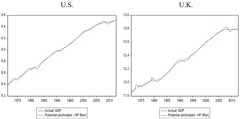
is the Hodrick and Prescott (1997) filter (HP). HP is widely used by international organisations and institutions such as the IMF and the European Central Bank which

extracts from a time-series yt the growth component, trend, Tt. The real GDP (seasonally

adjusted) in natural logs is used as a proxy for the actual real output. For the U.S., data come from the Federal Reserve Bank of Philadelphia and for the U.K. from the Office of National Statistics (ONS). Before applying the filter we backcast and forecast our data by 12 data points with an AR(4) model in order to correct for the end-of-sample problem that filters such as the HP present (e.g. Clausen and Meier (2005)).

U.S. U.K.

8.2 8.4 8.6 8.8 9.0 9.2 9.4 9.6

1975 1980 1985 1990 1995 2000 2005 2010

Actual GDP

Potential (estimated - HP filter) 11.8 12.0 12.2 12.4 12.6 12.8 13.0

1975 1980 1985 1990 1995 2000 2005 2010

Actual GDP

Potential (estimated - HP filter)

Figure 2.1: Actual and potential GDP (estimated with HP filter) of U.S. and U.K.

U.S. U.K.

-.05 .00 .05 .10 .15 .20

1975 1980 1985 1990 1995 2000 2005 2010

Output Gap Inflation rate

Interest rate (nominal)

-.05 .00 .05 .10 .15 .20 .25 .30

1975 1980 1985 1990 1995 2000 2005 2010

Output gap Inflation rate Interest rate (nominal)

14 Results

We report results for the Double maximum (UDmax and WDmax) test and the supF(k)

of 0 vs k number of breaks. The indicated change points are estimated using the global

minimisation, where the maximum number of breaks is set to 8.

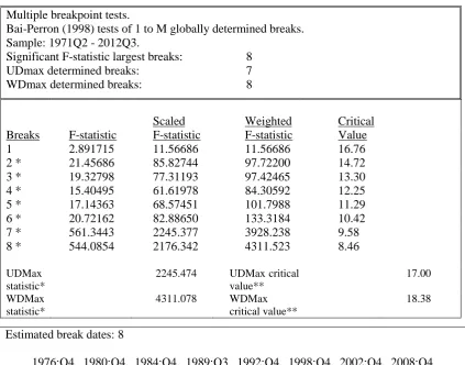
Table 2.1: Bai and Perron (1998) multiple breakpoint tests of the U.S. policy rule

Multiple breakpoint tests.

Bai-Perron (1998) tests of 1 to M globally determined breaks. Sample: 1971Q2 - 2012Q3.

Significant F-statistic largest breaks: 8

UDmax determined breaks: 7

WDmax determined breaks: 8

Scaled

Weighted

Critical

Breaks F-statistic F-statistic F-statistic Value

1 2.891715 11.56686 11.56686 16.76

2 * 21.45686 85.82744 97.72200 14.72

3 * 19.32798 77.31193 97.42465 13.30

4 * 15.40495 61.61978 84.30592 12.25

5 * 17.14363 68.57451 101.7988 11.29

6 * 20.72162 82.88650 133.3184 10.42

7 * 561.3443 2245.377 3928.238 9.58

8 * 544.0854 2176.342 4311.523 8.46

UDMax statistic*

2245.474 UDMax critical value**

17.00

WDMax statistic*

4311.078 WDMax critical value**

18.38

Notes: Included observations: 166. Break test options: trimming 0.10, max. breaks 8, sig. level 0.05. Test statistics employ HAC covariances (Pre-whitening with lags = 1, Quadratic-Spectral kernel, Andrews bandwidth). Allow heterogeneous error distributions across breaks.

* Significant at the 0.05 level.

** Bai-Perron (Econometric Journal, 2003) critical values.

The estimated break of 1980:Q4 is not far from the date at which Volcker took over the Chairmanship of the Fed, and this period is also reported as a regime shift in the majority of the economic literature. Qin and Enders (2008) estimate the interest rate reaction function of the U.S. before and after Greenspan period and conclude that the Taylor rule specification that best fits the data differs, implying a change in the

Estimated break dates: 8

15

monetary policy. Our test captures this change, although it suggests that this took place one year later. Regarding the 1984:Q4 break, it is difficult to historically clarify the significance and importance of this date. Nevertheless, the ‘Plaza Agreement’ between the U.S. and other major economies, which led to the devaluation of the U.S. dollar, could be an event causing this break (Duffy and Engle-Warnick, 2006). The 1989:Q3 break estimated by the test is documented in Goodfriend (2002) as a period of rising inflation, with the Fed maintaining a neutral response and hesitation against this inflationary surge. Data also indicate an increase in wage inflation, a fall in the unemployment rate, and somewhat steady productivity growth around this period. The next structural break reported by the test is at the end of 1992. Goodfriend (2002) describes the 1990:Q3–1994:Q1 period as a war, recession, and disinflation period. The Gulf War, the significant increase in oil prices by 20 dollars per barrel, and the price drop due to the recession that the war brought were the main events affecting not only the U.S. economy in that period. During that period, there was a remarkable decrease in the federal funds rate from 6% to 3% by the end of 1992, an increase in the real output growth rate, and a ceaseless upward trend in the unemployment rate of around 8% by June 1992. This period is documented by Goodfriend (2002) as the ‘jobless recovery’. In 1998:Q4, Bai and Perron (1998) (BP) test estimates the next structural break after the birth of the euro. As Goodfriend (2002) mentions, the period of 1996–1999, the U.S. economy presented a ‘boom’ in its productivity growth of 2.4% per year, on average, increasing household income and spending. These auspicious economic conditions were followed by a burst in technological advances and investment by firms in an attempt to modernise their assets, expand production even more, and hire a more

educated and productive labour force in order to become more competitive.6 The U.S.

invasion of Iraq in March 2003, following the attack on the World Trade Centre on 11 September 2001, in which approximately 800,000 people lost their jobs causing an increase in government spending and a decline in consumer spending, could be the reason why the BP test estimates 2002:Q4 as a structural change in monetary policy. The last break is located in 2008:Q4, when the financial crisis and the credit crunch started in the U.S. housing sector and the Fed dropped interest rates close to the zero lower bound.

6 _{Goodfriend (2002) reports two other events during that period: the financial crisis in East Asia and the}

16

Regarding the U.K., we report the estimated structural break dates obtained from the BP test with the maximum number of breaks equal to five. Evidence is less clear for the

number of breaks since UDmax suggests two breaks, while WDmax suggests four, and

supFT(5) suggests five breaks.

Table 2.2: Bai and Perron (1998) multiple breakpoint tests of the U.K. policy rule

Multiple breakpoint tests.

Bai-Perron tests of 1 to M globally determined breaks. Sample: 1971Q2 - 2012Q3.

Significant F-statistic largest breaks: 5

UDmax determined breaks: 2

WDmax determined breaks: 4

Scaled Weighted Critical

Breaks F-statistic F-statistic F-statistic Value

1 2.317696 9.270784 9.270784 16.19

2 * 5.897055 23.58822 27.73372 13.77

3 * 5.244817 20.97927 27.90915 12.17

4 * 4.902727 19.61091 29.42545 10.79

5 * 4.136487 16.54595 29.46963 9.09

UDMax statistic

23.5882 UDMax critical value**

16.37

WDMax statistic*

29.4696 WDMax

critical value**

17.83

Notes: Included observations: 166. Break test options: trimming 0.10, max. breaks 8, sig. level 0.05. Test statistics employ HAC covariances (Pre-whitening with lags = 1, Quadratic-Spectral kernel, Andrews bandwidth). Allow heterogeneous error distributions across breaks.

* Significant at the 0.05 level.

** Bai-Perron (Econometric Journal, 2003) critical values.

The first estimated break that supFT(5) suggests is in 1978:Q2, when ten months

previously, a new regime began with the election of Thatcher’s Conservative government. The first quarter of 1987 is the next suggested break, when, the informal link between sterling and the deutsche mark occurred, along with the very close relationship between U.K. and German monetary policy. The third change is estimated

Estimated break dates: 5

17

in 1993:Q4, when, in the previous year, the government announced the new policy of inflation targeting; for this reason, this date is used by the majority of studies to test the regime shifts of U.K. monetary policy. The forth break is in 2000:Q2, when inflation dropped. The last break is in 2007:Q1, at the beginning of the credit crunch.

2.3 Motivation and TVP-BVAR forecasting model

Engel and West (2005) use an asset-pricing framework to explain the random walk behaviour of the exchange rate. They argue that the exchange rate can be expressed as the discounted sum of the current observable and unobservable fundamentals, and has the following form:

(1 ) ( ) ( _{2, 2,} )

0 ,

1 , 1 0

j t j t t j

j j

t j t t j

j

t b b E f v b b E f v

s _{ }



 

 



 

 







where s is the log of the exchange rate, b is the discount factor, f collects the observable

fundamentals, and v the unobservable fundamentals while the ‘no-bubbles’ condition

for the expected spot exchange rate is assumed. They show that, if at least one forcing fundamental is I(1) and the discount factor is close to 1, then the exchange rate will move approximately like a random walk, while the correlation between exchange rate returns and changes of the macro fundamentals is very small. Their second finding, which is our main motivation in this chapter, comes from the Granger-causality analysis. Their in-sample analysis provides evidence that nominal exchange rate changes Granger-cause the macro fundamentals and this causality is much stronger than the other way around. Hence, they reach the conclusion that there is a link between them, such that the exchange rates can help forecasting the macroeconomic fundamentals.

Largely inspired by the second finding of EW05, we extend their work and we forecast the major macroeconomic fundamentals (output gap, inflation, and real exchange rate) by building an out-of-sample real-time forecasting exercise employing

a TVP-BVAR model.7 More specifically, we use the Taylor rule-based forecasting

7 _{As Rossi (2013b) mentions, the empirical evidence of in-sample predictability does not necessarily}

18

model as in Molotdsova and Papell (2009). To do so, we use equation (2.4) as the monetary policy for the home country (U.S.) and the same for the foreign country (U.K.)

incorporating the real exchange rate (q_t) as well. So, we can re-write the policy rule:

Home country: t t

gap t y t

t y i

i _   _1 , (2.6)

where _ (1), y (1) and (1). Regarding the foreign country:

Foreign country: i_tf f _f_tf _yfy_tfgap_qfq_tf fi_tf_1_tf, (2.7)

where f denotes the terms of the foreign country, _qf (1f) and q_tf is the real

exchange rate of the foreign country assuming that this country is targeting the Purchasing Power Parity (PPP) level of the exchange rate (Molotdsova and Papell,

2009).8 Hence, to derive the Taylor rule-based forecasting equation, the interest rate

reaction function of the foreign country is subtracted from that of the home country.

Assuming that the uncovered interest rate parity (UIP) holds, _t





following forecasting equation is derived:9

 1        1 1 t1

f t f t f t f q fgap t f y gap t y f t f t

t a y y q i i u

s         , (2.8)

where (f) and u_t1 is the error term. Equation (2.8) is our starting point. In

other words, we incorporate this theory-based model into a vehicle that will allow us to forecast the Taylor rule fundamentals. We decide that the vehicle should be a VAR model since this can develop and elaborate theory-based simultaneous forecasting equations. First of all, VARs have become the workhorse model for multivariate analysis and for macroeconomic forecasting exercises since the pioneering work of Sims (1980). Some features of this vehicle are its simplicity, flexibility and ability to fit

estimating the model in hand and then conducting a traditional Granger-causality test, checking the significance of the estimated parameters using a simple t-test. On the other hand, out-of-sample predictability is tested by splitting the sample into two parts. The in-sample part is used for estimations and to generate forecasts, while the out-of-sample part is used to evaluate them using the appropriate loss functions.

8 _{The real exchange rate is defined as the nominal FX rate plus the foreign price level minus the home}

price level, where variables are in natural logarithms.

9 _{Linking the interest rate differential with the exchange rates is discussed by Molodtsova and Papell}

19

the data through the rich over-parameterisation that entails the danger of imprecise inference and failure to summarise the dynamic correlation patterns among the observables and their future paths, leading to poor forecasts. ‘Shrinkage’ has been the

solution to this over-fitting problem, by imposing prior constraints and beliefs on the

model’s parameters, (see, for example, the Minnesota prior used by Litterman (1979)

and Doan et al. (1984)). Bayes’ theorem then provides the optimal way of combining

all the available information coming from the data and the prior beliefs leading to the posterior inference and probably more accurate predictions.

As discussed in the previous section, Taylor rule relationships suffer from structural changes and non-linearities. So, for the purpose of our forecasting exercise, we employ a time-varying parameters Bayesian VAR model (TVP-BVAR), in order to account for the changes in the monetary policy rules over time. This kind of model assumes a constant covariance matrix (homoscedastic TVP-BVAR) and treats all the variables as endogenous. Similar heteroscedastic TVP-BVAR models, where the time variation derives from both parameters and the variance-covariance matrix of the models’

innovations, have been used in Primiceri (2005) and D’Agostino et al. (2013), while the

homoscedastic models have been used by Sarantis (2006) and Byrne et al. (2016).

Hence, for our forecasting exercise, a homoscedastic TVP-BVAR model as in Korobilis (2013) has been selected. Keeping Korobilis’s (2013) notation, the reduced form TVP-BVAR can be written in the following linear specification:

y_t c_t  B_1,ty_t1B_2,ty_t2....B_p,ty_tp u_t, (2.9)

where p is the number of lags, yt is an m×1 vector of t = t,...,T observations of the

dependent variables, B matrices collect the coefficients, errors ut ~Nm(0,) where Σ

is a constant covariance matrix of m×m dimensions and m is the number of variables.

Re-writing the model in a linear state-space form:

y_t z_t_t _t (2.10)

t t1t (2.11)

equation (2.10) is the measurement equation where z_t I_m x_t I_m





20

walk state equation of the parameters, βt is an n1 state vector

 

 





, '

, 1 '

,...,

, _{t pt}

t vecB vecB

c of parameters, _t ~ N(0,Q), where Q is an nn

covariance matrix, and  ~ N(0,), where Σ is an mm covariance matrix of the

model. It is assumed that _t and _t are not correlated at all lags and leads. Kim and

Nelson (1999) show how TVP models can be expressed in a state-space form and how the unobserved states of the time-varying parameters can be estimated via the Kalman filter.

As discussed earlier, we want to bring the theory-based model (eq. 2.8) into the TVP-BVAR vehicle, which will allow us to forecast the Taylor rule fundamentals. Therefore, the vector of dependent variables of our model is represented by:





 _{ }f

t t f t f t t fgap t gap t t

t s y y q i i

Y , , , , , , 1, 1 , where (Δs) is the nominal exchange rate

change, (ygap) is the output gap, (π) is the inflation rate, (q) is the real exchange rate, and

(i) is the nominal interest rate set by the monetary authorities (with a period lag due to

the gradual adjustment to the target level). In order to investigate the predictive content of the exchange rates, we want to allow a priori only the exchange rate changes to give their predictive power, along with the first own lag of each dependent variable. The Bayesian approach treats all coefficients as random variables by assigning a prior distribution to them and allowing the data likelihood to determine their posterior values. So, we decide to assign an uninformative normal prior for the constants and the fundamentals that we allow them to a priori predict, and a very tight normal prior for the predictors that we want to restrict.

Priors

Regarding the random walk transition equation, we practically need to set the initial

condition (starting values for the Kalman filter) of βt.According to Korobilis (2013),

priors for the parameters do not need to be specified in every time period since this is

implicitly defined recursively as _t ~N(_t1,Q). Given the purpose of our forecasting

exercise, we use a non-informative normal prior of ₀ ~N(0,102) for the variables

that we allow to draw predictive power, and a tight normal prior of ₀ ~ N(0,0.012)

21

inverse Wishart prior has been set as: ~IW(J1,v), with non-informative

hyperparameters (J  0), where J is the scale matrix and v is thedegrees of freedom

as in Koop and Korobilis (2009). For the covariance matrix Q,we impose an inverse

Wishart prior, Q~IW(R1,), where  (n1)2 is the degrees of freedom (n is the

number of parameters in the state vector) and Rk_RI_n , where k_R is the scaling factor

and equal to 0.0001, as used in Primiceri (2005). Cogley and Sargent (2002) suggest that this kind of scaling factor should be used, since time-varying parameters should vary smoothly and not change sharply over time. Details about the posterior distributions, the Kalman filter, and the smoothing process can be found in Appendix B.

As a standard practice in the forecasting exercises, we also employ a BVAR(1) model with the so-called Minnesota prior (Doan et al. 1984) and a standard VAR(1) model estimated via OLS to forecast the macro-fundamentals, while all the aforementioned candidate models are compared with the driftless random walk benchmark model. We use 1 number of lags, as BIC recursively suggests. Details about the BVAR specification and the Minnesota prior can be found in Appendix B.

2.4 Data and real-time forecasting exercise

It is well known that data such as output, price level indices, money stock, and others, are continuously revised by statistical offices due to changes in the definition of the variables (e.g. GNP to GDP), or just because statistical agencies have acquired additional information and current data are being updated. Hence, a real-time dataset is an important ‘tool’, especially for researchers who conduct out-of-sample forecasting

exercises. Among others, Croushore and Stark (2001), Croushore (2006), Orphanides (2001, 2003), Molodtsova and Papell (2009), and Faust, Rogers and Wright (2003) have studied the importance of using real-time data in several forecasting and estimation exercises and conclude that the predictive ability of the forecasting model is enhanced

by using real-time data.Also, Clements (2012) pinpoints the fact that findings about

22

to the forecaster only at the time he was making the forecasts.10 _{Variables such as}

nominal exchange rates and nominal interest rates are never revised.

We use quarterly data from 1971:Q2 to 2012:Q3 for the two countries (U.S. and U.K.). The real GDP (seasonally adjusted) is used as a proxy for the U.S. output, extracted from the Fed of Philadelphia, and for the real GDP of U.K., data extracted from the ONS. For both countries, the output gap is measured using the HP filter. Before we apply the filter, we backcast and forecast our data by 12 datapoints with an AR(4)

model. As regards the inflation rate, we compute it as πt = GDP deflatort – GDP

deflatort-4 (GDP deflator in natural logs). For the data that is not revised, we use the

Pacific Exchange Rate Service website to extract the nominal USD/GBP exchange

rate.11 We calculate the real GBP/USD exchange rate as the nominal GBP/USD

exchange rate plus the log of the U.S. price level minus the log of the U.K. price level. The USD/GBP exchange rate is defined as the U.S. dollar price of a British pound.

Regarding the interest rates, it would not be wise to use the effective Federal fund rate and the Official Bank rate as a proxy for the nominal interest rates since both figures hit the zero lower bound (ZLB) at the end of 2008. Instead, there are studies that suggest the long-term interest rates as an alternative monetary policy instrument. McCough et al. (2005) characteristically mention that the long-term rates might be a physical substitute as they are highly related to the future expected path of the short-term interest rates, while Jones and Kulish (2013) show that long-term rates are good instruments for conducting monetary policy and sometimes performing better than the standard Taylor rules. Also, Chinn and Meredith (2004) provide empirical evidence to show that testing UIP model using interest rates on longer-maturity bonds, leads to better in-sample results consistent with the UIP theory. On the other hand, Wu and Xia (2016) construct a new measure called shadow rate, approximating the effective Federal fund rate. By using a Gaussian affine term structure model, they generate a shadow rate allowed for taking negative values, and replace the federal fund rate time-series with this shadow rate for the period where economy is at the ZLB. They find that this shadow rate is highly correlated with the federal fund rate before 2009, interacting with the macro fundamentals in the same manner as federal fund rate did with them historically. In this

10 _{We should note that in real-time datasets there is always one period lag between the vintage date and}

the last observation of that vintage. So, assuming, for example, the 2000:Q1 vintage, the last observation of that vintage is at 1999:Q4.

23

study we opt to use the 10-year Treasury bond rates as a proxy for the nominal interest rates.

2.4.1 Forecast implementation and evaluation

For the out-of-sample forecasting exercise, we consider the recursive scheme along with the rolling scheme as a robustness check. In the recursive scheme, the model is estimated for the period 1971:Q2–1989:Q4 (using data from the 1990:Q1 vintage) and

iterated forecasts are generated and stored for h periods ahead, where h =1-, 2-, 3-, and

4-quarters-ahead horizon. Then, data in vintage 1990:Q2 is used and the model is

re-estimated again, with forecasts for h periods ahead being computed again. This process

is repeated until the whole dataset is exhausted. We explore the robustness of our results with respect to different forecasting scheme. Hence, the rolling scheme is also used, where estimations of the model are made with a fixed-size rolling window, which we choose to set at 15 years (i.e. 61 most recent observations available at the time we conduct the forecasts).

According to D’Agostino et al.(2013) and Korobilis (2013), if we rewrite our model

in the form below, we can derive the standard forecasting formula using the iterative method. So, given the companion form of our TVP-BVAR model:

yt = ct + Btyt-1 + εt ,

where yt =













 ,0,....,0 t

c and Bt = 

         m p m p m t p t p t I B B B ) 1 ( ) 1 ( , , 1 , 1 0 ... ,

then iterated h-step ahead forecasts can be obtained according to the following formula:

E(yt+h) =



  1 0 h i

Btict + Bth yt-1 . (2.12)

Following Korobilis (2013), we plug into the above formulas the values of the last

known coefficients in sample

 

It is a standard practice to evaluate the performance of a forecasting model using the root mean square forecast error (RMSFE) and the mean absolute forecast error (MAFE).

24

observed (A) value as a squared term, and the square root is taken and averaged over

the total out-of-sample period. The second method measures the magnitude of the forecast error, where absolute values are taken and averaged over the full forecasting period.





0 1 2 1 1 0                   



, (2.13)







, (2.14)

where τ0 corresponds to the last observation of the in-sample period and τ1 is the end of

the forecasting period. Our forecasts are compared with the corresponding figure observations published the next quarter vintage. Most of the time, we are interested in reporting the relative RMSFE and the relative MAFE by dividing the RMSFE and the MAFE of the candidate forecasting model by those of the benchmark forecasting model. The benchmark model that we choose for all the variables is the driftless random walk (RW). The same benchmark model has been used by Korobilis (2013), who forecasts the U.K. inflation, unemployment, and interest rate. The driftless RW assumes that









0

t

y

y

E

forecast error o

h t t o h t t h t RW t h

t y y y y

fe_ |  ˆ_{ |}  _   _ , where

o h t

y

(realisation) at t+h. Another standard practice in the forecasting literature is to test

25

2.5 Empirical results

The following tables report the relative RMSFE and MAFE, where a ratio below 1 denotes that the candidate model (TVP-BVAR, BVAR or VAR) outperforms the

benchmark model in out-of-sample accuracy. The CW test is also reported in the

following tables at different levels of significance. The results of the recursive scheme are reported first, and then robustness is checked using the rolling estimation scheme.

Recursive scheme

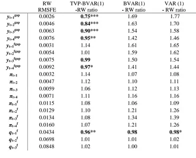
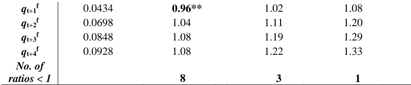
Table 2.3 presents the results of the forecasts’ evaluation based on the RMSFE. In seven out of 20 cases, TVP-BVAR outperforms the RW, while in only two cases, BVAR and VAR forecast better than the benchmark. More specifically, the TVP model improves upon the RW when forecasting the U.S. output gap at all horizons, the U.K. output gap for 3- and 4-quarters-ahead, and the U.K. real exchange rate at 1-period-ahead. For the majority of these cases, the results are highly significant, as the CW test indicates.

Table 2.3: Relative RMSFE of candidate models for h = 1, 2, 3 and 4 periods ahead

RW RMSFE

TVP-BVAR(1)

-RW ratio

BVAR(1)

- RW ratio

VAR (1)

- RW ratio

yt+1gap _{0.0026 0.75*** 1.69 1.77}

yt+2gap _{0.0046 0.84*** 1.63 1.70}

yt+3gap _{0.0063 0.90*** 1.54 1.58}

yt+4gap _{0.0076 0.95** 1.42 1.46}

yt+1fgap _{0.0031 1.14 1.61 1.65}

yt+2fgap _{0.0054 1.01 1.59 1.62}

yt+3fgap _{0.0075 0.99 1.50 1.54}

yt+4fgap _{0.0092 0.97* 1.41 1.44}

πt+1 0.0032 1.14 1.07 1.08

πt+2 0.0047 1.12 1.10 1.11

πt+3 0.0059 1.06 1.12 1.13

πt+4 0.0071 1.11 1.16 1.16

πt+1f _{0.0115 1.08 1.06 1.09}

πt+2f _{0.0129 1.10 1.21 1.26}

πt+3f _{0.0134 1.08 1.34 1.39}

πt+4f _{0.0160 1.07 1.21 1.26}

qt+1f _{0.0434 0.96** 0.98 0.98*}

qt+2f _{0.0698 1.01 1.01 1.02}

26

qt+4f _{0.0928 1.02 0.98 0.98}

No. of ratios < 1

7 2 2

Notes: The above results are obtained via recursive estimations. The first column shows the RMSFE of the driftless random walk. The second, third and fourth columns report the relative RMSFE, where a ratio less than 1 (in bold) indicates that the candidate model generates lower RMSFE than the RW. Asterisks indicate that the null hypothesis of equal predictive accuracy (one-sided CW test) is rejected against the alternative of outperforming the benchmark model at the 1% (***), 5% (**) and 10% (*) significance levels. The superscript f denotes the variables of the U.K., while the rest fundamentals belong to the U.S.

The results for the U.S. inflation are pessimistic, with the RW model always generating lower RMSFE than our model. Stock and Watson (2007, 2008) admit that inflation is difficult to forecast, especially in large samples. Nevertheless, they show

that a backward-looking Phillips curve (with autoregressive distributed lag – ADL

specification) delivers better inflation forecasts than an AR(AIC) model for the U.S. in both short and long horizons, although these results are heavily sample dependent. Also, the Bayesian model averaging models used by Wright (2009) and Nikolsko-Rzhevskyy (2011), and the TVP-BVAR model with stochastic volatility used by D’Agostino et al. (2013), clearly outperform the random walk at any horizon when forecasting the U.S. inflation rate. Regarding the forecasting performance of the BVAR(1) and VAR(1) models, predictions look very poor compared to the benchmark model. Using the relative MAFE, the results remain somewhat the same, as reported in Table 2.4.

Table 2.4: Relative MAFE of candidate models for h = 1, 2, 3 and 4 periods ahead

RW MAFE

TVP-BVAR(1)

-RW ratio

BVAR(1)

- RW ratio

VAR (1)

- RW ratio

yt+1gap _{0.0019 0.75 1.80 1.87}

yt+2gap _{0.0035 0.84 1.76 1.82}

yt+3gap _{0.0048 0.88 1.63 1.68}

yt+4gap _{0.0060 0.91 1.49 1.53}

yt+1fgap _{0.0022 1.12 1.72 1.76}

yt+2fgap _{0.0038 1.01 1.79 1.84}

yt+3fgap _{0.0054 0.98 1.73 1.78}

yt+4fgap _{0.0065 0.95 1.69 1.73}

πt+1 0.0025 1.05 1.06 1.07

πt+2 0.0037 1.09 1.10 1.11

πt+3 0.0048 1.04 1.11 1.11

πt+4 0.0058 1.10 1.14 1.14

πt+1f _{0.0071 1.08 1.13 1.16}