Tomislav Stankovski1,2, Tiago Pereira3,4, Peter V. E. McClintock2, and Aneta Stefanovska2 1 Faculty of Medicine, Ss Cyril and Methodius University, 50 Divizija 6, Skopje 1000, Macedonia 2 Department of Physics, Lancaster University, Lancaster, LA1 4YB, United Kingdom
3
Department of Mathematics, Imperial College London, London SW7 2AZ, United Kingdom and 4
Institute of Mathematical and Computer Sciences, University of S˜ao Paulo, S˜ao Carlos 13566-590, Brazil
(Dated: November 14, 2017)
The dynamical systems found in Nature are rarely isolated. Instead they interact and influence each other. The coupling functions that connect them contain detailed information about the functional mechanisms underlying the interactions and prescribe the physical rule specifying how an interaction occurs. Here, we aim to present a coherent and comprehensive review encompassing the rapid progress made recently in the analysis, understanding and applications of coupling functions. The basic concepts and characteristics of coupling functions are presented through demonstrative examples of different domains, revealing the mechanisms and emphasizing their multivariate nature. The theory of coupling functions is discussed through gradually increasing complexity from strong and weak interactions to globally-coupled systems and networks. A variety of methods that have been developed for the detection and reconstruction of coupling functions from measured data is described. These methods are based on different statistical techniques for dynamical inference. Stemming from physics, such methods are being applied in diverse areas of science and technology, including chemistry, biology, physiology, neuroscience, social sciences, mechanics and secure communications. This breadth of application illustrates the universality of coupling functions for studying the interaction mechanisms of coupled dynamical systems.
PACS numbers: 05.45.Xt, 05.45.-a, 05.45.Tp, 02.50.Tt
Contents
I. Introduction 2
A. Coupling functions, their nature and uses 2 B. Significance for interacting systems more generally 3
1. Physical effects of interactions: Synchronization, amplitude and oscillation death 3 2. Coupling strength and directionality 4 3. Coupling functions in general interactions 5
II. Basic Concept of Coupling Functions 5
A. Principle meaning 5
1. Generic form of coupled systems 5 2. Coupling function definition 5 3. Example of coupling function and synchronization 6
B. History 7
C. Different domains and usage 8
1. Phase coupling functions 8
2. Amplitude coupling functions 9 3. Multivariate coupling functions 10 4. Generality of coupling functions 11 D. Coupling functions revealing mechanisms 12 E. Synchronization prediction with coupling functions 13
F. Unifying nomenclature 14
III. Theory 14
A. Strong interaction 14
1. Two coupled oscillators 14
2. Comparison between approaches 18
B. Weak regime 18
1. Stable Periodic Orbit and its phase 19 2. Coupling function and phase reduction 20 3. Synchronization with external forcing 20
4. Phase response curve 21
5. Examples of the phase sensitivity function 22 C. Globally coupled oscillators 23 1. Coupling functions leading to multistability 23
2. Designing coupling functions for cluster states and
chimeras 24
3. Coupling functions with delay 24
4. Low dimensional dynamics 24
5. Noise and nonautonomous effects 25
D. Networks of oscillators 26
1. Reduction to phase oscillators 26 2. Networks of chaotic oscillators 26
IV. Methods 27
A. Inferring coupling functions 27 B. Methods for coupling function reconstruction 29 1. Modeling by least-squares fitting 29 2. Dynamical Bayesian inference 30 3. Maximum likelihood estimation: multiple-shooting 31 4. Random phase resetting method 33 5. Stochastic modeling of effective coupling functions 33 6. Comparison and overview of the methods 34 C. Towards coupling function analysis 35 D. Connections to other methodological concepts 36 1. Phase reconstruction procedures 36 2. Relation to phase response curve in experiments 36 3. General effective connectivity modeling 37
V. Applications and Experiments 38
A. Chemistry 38
B. Cardiorespiratory interactions 40
C. Neural coupling functions 42
D. Social sciences 43
E. Mechanical coupling functions 44
F. Secure communications 45
VI. Outlook and Conclusion 46
A. Future directions and open questions 46
1. Theory 46
2. Methods 46
3. Analysis 47
5. Applications 47
B. Conclusion 48
Acknowledgments 48
References 48
I. INTRODUCTION
A. Coupling functions, their nature and uses
Interacting dynamical systems abound in science and technology, with examples ranging from physics and chemistry, through biology and population dynamics, to communications and climate (Haken, 1983; Kuramoto,
1984; Pikovsky et al., 2001; Strogatz, 2003; Winfree,
1980).
The interactions are defined by two main aspects: structure and function. The structural links determine the connections and communications between the sys-tems, or the topology of a network. The functions are quite special from the dynamical systems viewpoint, as they define the laws by which the action and co-evolution of the systems are governed. The functional mecha-nisms can lead to a variety of qualitative changes in the systems. Depending on the coupling functions, the re-sultant dynamics can be quite intricate, manifesting a whole range of qualitatively different states, physical ef-fects, phenomena and characteristics, including synchro-nization (Acebr´on et al., 2005; Kapitaniak et al., 2012;
Lehnertz and Elger,1998;Pikovskyet al.,2001), oscilla-tion and amplitude death (Koseskaet al.,2013a;Saxena et al.,2012), birth of oscillations (Pogromskyet al.,1999;
Smale,1976), breathers (MacKay and Aubry,1994), co-existing phases (Keller et al., 1992), fractal dimensions (Aguirre et al., 2009), network dynamics (Arenas et al.,
2008;Boccalettiet al.,2006), and coupling strength and directionality (Hlav´aˇckov´a´a-Schindleret al., 2007; Mar-wan et al., 2007; Rosenblum and Pikovsky, 2001; Ste-fanovska and Braˇciˇc,1999). Knowledge of such coupling function mechanisms can be used to detect, engineer or predict certain physical effects, to solve some man-made problems and, in living systems, to reveal their state of health and to investigate changes due to disease.
Coupling functions possess unique characteristics car-rying implications that go beyond the collective dynamics (e.g. synchronization or oscillation death). In particular, the form of the coupling function can be used, not only to understand, but also to control and predict the inter-actions. Individual units can be relatively simple, but the nature of the coupling function can make their col-lective dynamics particular, enabling special behaviour. Additionally, there exist applications which depend just and only on the coupling functions, including examples of applications in social sciences and secure communication. Given these properties, it is hardly surprising that coupling functions have recently attracted considerable attention within the scientific community. They have
mediated applications, not only in different subfields of physics, but also beyond physics, predicated by the de-velopment of powerful methods enabling the reconstruc-tion of coupling funcreconstruc-tions from measured data. The re-construction within these methods is based on a vari-ety of inference techniques, e.g. least squares and ker-nel smoothing fits (Kralemann et al., 2013a; Rosen-blum and Pikovsky,2001), dynamical Bayesian inference (Stankovskiet al.,2012), maximum likelihood (multiple-shooting) methods (Tokudaet al.,2007), stochastic mod-eling (Schwabedal and Pikovsky,2010) and the phase re-setting (Gal´anet al.,2005;Levnaji´c and Pikovsky,2011;
Timme,2007).
Both the connectivity between systems, and the asso-ciated methods employed for revealing it, are often dif-ferentiated into structural, functional and effective con-nectivity (Friston,2011;Park and Friston,2013). Struc-tural connectivity is defined by the existence of a phys-ical link, like anatomphys-ical synaptic links in the brain or a conducting wire between electronic systems. Func-tional connectivity refers to the statistical dependences between systems, like for example correlation or coher-ence measures. Effective connectivity is defined as the influence one system exerts over another, under a par-ticular model of causal dynamics. Importantly in this context, the methods used for the reconstruction of cou-pling functions belong to the group of effective connec-tivity techniques i.e. they exploit a model of differential equations and allow for dynamical mechanisms – like the coupling functions themselves – to be inferred from data.
Coupling function methods have been applied widely (Fig. 1), and to good effect: inchemistry, for understand-ing, effectunderstand-ing, or predicting interactions between oscilla-tory electrochemical reactions (Blaha et al., 2011; Kiss et al., 2007; Kori et al., 2014; Miyazaki and Kinoshita,
2006; Tokuda et al., 2007); in cardiorespiratory physi-ology (Iatsenko et al., 2013; Kralemann et al., 2013a;
Stankovskiet al., 2012) for reconstruction of the human cardiorespiratory coupling function and phase resetting curve, for assessing cardiorespiratory time-variability and for studying the evolution of the cardiorespiratory cou-pling functions with age; in neuroscience for revealing the cross-frequency coupling functions between neural oscillations (Stankovski et al., 2015); in social sciences for determining the function underlying the interactions between democracy and economic growth (Ranganathan et al.,2014); formechanicalinteractions between coupled metronomes (Kralemannet al.,2008); and insecure com-municationswhere a new protocol was developed explic-itly based on amplitude coupling functions (Stankovski et al.,2014).
In parallel with their use to support experimental work, coupling functions are also at the centre of in-tense theoretical research (Acebr´on et al., 2005; Craw-ford, 1995; Daido, 1996a; Strogatz, 2000). Particular choices of coupling functions can allow for a multiplicity of singular synchronized states (Komarov and Pikovsky,
Figure 1 (color online). Examples of coupling functions used in chemistry, cardiorespiratory physiology and secure commu-nications, to demonstrate their diversity of applications. (a) Coupling functions used for controlling and engineering the interactions of two (left) and four (right) non-identical elec-trochemical oscillations. (b) Human cardiorespiratory cou-pling functionQereconstructed from the phase dynamics the heartϕe and respiration ϕr phases. (c) Schematic descrip-tion of the coupling funcdescrip-tion encrypdescrip-tion protocol. Multi-ple information signals are encrypted by modulating the pa-rameters of linearly-independent coupling functions between (chaotic) dynamical systems at the transmitter. These appli-cations are discussed in detail in Sec. V. Fig. 1(a) is fromKiss et al.(2007), (b) fromKralemannet al.(2013a) and (c) from Stankovskiet al.(2014).
coherence in complex networks of non-identical oscilla-tors (Luccioli and Politi,2010;Pereiraet al.,2013;Ullner and Politi,2016) and for the formation of waves and anti-waves in coupled neurons (Urban and Ermentrout,2012). Coupling functions play important roles in the phenom-ena resulting from interaction such as synchronization (Daido,1996a; Kuramoto, 1984;Maiaet al.,2015), am-plitude and oscillation death (Aronsonet al.,1990; Kos-eskaet al.,2013a;Schneideret al.,2015;Zakharovaet al.,
2014), the low-dimensional dynamics of ensembles (Ott and Antonsen,2008;Watanabe and Strogatz,1993), and clustering in networks (Ashwin and Timme, 2005; Kori et al.,2014). The findings of these theoretical works are fostering further the development of methods for coupling function reconstruction, paving the way to additional
ap-plications.
B. Significance for interacting systems more generally
An interaction can result from a structural link through which causal information is exchanged between the system and one or more other systems (Haken,1983;
Kuramoto, 1984; Pikovsky et al., 2001; Strogatz, 2003;
Winfree, 1980). Often it is not so much the nature of the individual parts and systems, but how they inter-act, that determines their collective behaviour. One ex-ample is circadian rhythms, which occur across different scales and organisms (DeWoskinet al., 2014). The sys-tems themselves can be diverse in nature – for example, they can be either static or dynamical, including oscilla-tory, nonautonomous, chaotic, or stochastic characteris-tics (Gardiner,2004;Katok and Hasselblatt,1997; Kloe-den and Rasmussen, 2011; Landa, 2013; Strogatz, 2001;
Suprunenkoet al.,2013). From the extensive set of pos-sibilities, we focus in this review on dynamical systems, concentrating especially on nonlinear oscillators because of their particular interest and importance.
1. Physical effects of interactions: Synchronization, amplitude and oscillation death
An intriguing feature is that their mutual interactions can change the qualitative state of the systems. Thus they can cause transitions into or out of physical states such as synchronization, amplitude or oscillation death, or quasi-synchronized states in networks of oscillators.
The existence of a physical effect is, in essence, defined by the presence of astable statefor the coupled systems. Their stability is often probed through a dimensionally-reduced dynamics, for example the dynamics of their phase difference or of the driven system only. By de-termining the stability of the reduced dynamics, one can derive useful conclusions about the collective behaviour. In such cases, the coupling functions describe how the stable state is reached and the detailed conditions for the coupled systems to gain or lose stability. In data analysis, the existence of the physical effects is often as-sessed through measures that quantify – either directly or indirectly – the resultant statistical properties of the state that remains stable under interaction.
The physical effects often converge to a manifold, such as a limit cycle. Even after that, however, coupled namical systems can still exhibit their own individual dy-namics, making them especially interesting objects for study.
(Lehnertz and Elger,1998), neuromuscular activity (Tass et al.,1998), chemistry (Kisset al., 2007; Miyazaki and Kinoshita,2006), the flashing of fireflies (Buck and Buck,
1968;Mirollo and Strogatz,1990) and ecological synchro-nization (Blasiuset al.,1999). Depending on the domain, the observable properties and the underlying phenomena, several different definitions and types of synchronization have been studied. These include phase tion, generalized synchronization, frequency synchroniza-tion, complete (identical) synchronizasynchroniza-tion, lag synchro-nization and anomalous synchrosynchro-nization (Arnholdet al.,
1999;Blasiuset al.,2003;Brown and Kocarev,2000; Er-mentrout, 1981; Eroglu et al., 2017; Kocarev and Par-litz, 1996; Kuramoto, 1984; Pecora and Carroll, 1990;
Pikovsky et al., 2001; Rosenblum et al., 1996; Rulkov et al.,1995).
Another important group of physical phenomena at-tributable to interactions are those associated with os-cillation and amplitude deaths (Bar-Eli, 1985; Koseska et al., 2013a; Mirollo and Strogatz, 1990;Prasad, 2005;
Schneider et al., 2015; Su´arez-Vargas et al., 2009; Za-kharova et al., 2013). Oscillation death is defined as a complete cessation of oscillation caused by the interac-tions, when an inhomogeneous steady state is reached. Similarly, in amplitude death, due to the interactions a homogeneous steady state is reached and the oscilla-tions disappear. The mechanisms leading to these two oscillation quenching phenomena are mediated by differ-ent coupling functions and conditions of interaction, in-cluding strong coupling (Mirollo and Strogatz,1990;Zhai et al.,2004), conjugate coupling (Karnataket al.,2007), nonlinear coupling (Prasad et al., 2010), repulsive links (Hens et al., 2013) and environmental coupling (Resmi et al., 2011). These phenomena are mediated, not only by the phase dynamics of the interacting oscillators, but also by their amplitude dynamics, where the shear am-plitude terms and the nonisochronicity play significant roles. Coupling functions define the mechanism through which the interaction causes the disappearance of the os-cillations.
There is a large body of earlier work in which physical effects, qualitative states, or quantitative characteristics of the interactions were studied, where coupling functions constituted an integral part of the underlying interac-tion model, regardless of whether or not the term was used explicitly. Physical effects are very important and they are closely connected with the coupling functions. In such investigations, however, the coupling functions themselves were often not assessed, or considered as en-tities in their own right. In simple words, such inves-tigations posed the question of whether physical effects occur; while for the coupling function investigations the question is rather how they occur. Our emphasis will therefore be on coupling functions as entities, on the ex-ploration and assessment of different coupling functions, and on the consequences of the interactions.
2. Coupling strength and directionality
The coupling strength gives a quantitative measure of the information flow between the coupled systems. In an information-theoretic context, this is defined as the trans-fer of information between variables in a given process. In a theoretical treatment the coupling strength is clearly the scaling parameter of the coupling functions. There is great interest in being able to evaluate the coupling strength, for which many effective methods have been designed (Bahraminasabet al.,2008;Chicharro and An-drzejak,2009;Faeset al.,2011;Jamˇseket al.,2010; Mar-wan et al., 2007; Mormannet al., 2000; Paluˇs and Ste-fanovska,2003;Rosenblum and Pikovsky,2001;Smirnov and Bezruchko, 2009; Staniek and Lehnertz, 2008; Sun et al., 2015). The dominant direction of influence, i.e. the direction of the stronger coupling, corresponds to the directionality of the interactions. Earlier, it was impossi-ble to detect the absolute value of the coupling strength, and a number of methods exist for detection only of the directionality through measurements of the relative mag-nitudes of the interactions – for example, when detect-ing mutual information (Paluˇs and Stefanovska, 2003;
Smirnov and Bezruchko, 2009; Staniek and Lehnertz,
2008), but not the physical coupling strength. The as-sessment of the strength of the coupling and its predom-inant direction can be used to establish if certain in-teractions exist at all. In this way, one can determine whether some apparent interactions are in fact genuine, and whether the systems under study are truly con-nected or not.
When the coupling function results from a number of functional components, its net strength is usually evalu-ated as the Euclidian norm of the individual components’ coupling strengths. Grouping the separate components, for example the Fourier components of periodic phase dynamics, one can evaluate the coupling strengths of the functional groups of interest. The latter could include the coupling strength from either one system or the other, or from both of them. Thus one can detect the strengths of the self, direct and common coupling components, or of the phase response curve (Faes et al., 2015; Iatsenko et al., 2013; Kralemann et al., 2011). In a very simi-lar way, these ideas can be generalized for multivariate coupling in networks of interacting systems.
It is worth noting that, when inferring couplings even from completely uncoupled or very weakly-coupled sys-tems, the methods will usually detect non-zero coupling strengths. This results mainly from the statistical prop-erties of the signals. Therefore, one needs to be able to ascertain whether the detected coupling strengths are genuine, or spurious, just resulting from the inference method. To overcome this difficulty, one can apply sur-rogate testing (Andrzejaket al.,2003;Kreuzet al.,2004;
surrogate signals should then reflect a “zero-level” of ap-parent coupling for the uncoupled signals. By compari-son, one can then assess whether the detected couplings are likely to be genuine. This surrogate testing process is also important for coupling function detection – one first needs to establish whether a coupling relation is genuine and then, if so, to try to infer the form of the coupling function.
3. Coupling functions in general interactions
The present review is focused mainly on coupling func-tions between interacting dynamical systems, and espe-cially between oscillatory systems, because most stud-ies to date have been developed in that context. How-ever, interactions have also been studied in a broader sense for non-oscillatory, non-dynamical, systems, spread over many different fields, including for example quan-tum plasma interactions (Marklund and Shukla, 2006;
Shukla and Eliasson, 2011), solid state physics (Farid,
1997; Higuchi and Yasuhara, 2003; Zhang, 2013), in-teractions in semiconductor superlattices (Bonilla and Grahn,2005), Josephson junction interactions (Golubov et al., 2004), laser diagnostics (Stepowski, 1992), inter-actions in nuclear physics (Guelfi et al., 2007; Mitchell et al.,2010), geophysics (Murayama,1982), space science (Feldstein, 1992; Lifton et al., 2005), cosmology (Baldi,
2011;Faraoni et al.,2006), biochemistry (Khramov and Bielawski, 2007), plant science (Doidy et al., 2012), oxygenation and pulmonary circulation (Ward, 2008), cerebral neuroscience (Liao et al., 2013), immunology (Robertson and Ghazal, 2016), biomolecular systems (Christen and Van Gunsteren, 2008; Dong et al., 2014;
Stamenovi´c and Ingber,2009), gap junctions (Weiet al.,
2004) and protein interactions (Gaballo et al., 2002;
Jones and Thornton, 1996; Okamoto et al., 2009; Teas-dale and Jackson, 1996). In many such cases, the in-teractions are different in nature. They are often struc-tural, and not effective connections in the dynamics; or the corresponding coupling functions may not have been studied in this context before. Even though we do not discuss such systems directly in this review, many of the concepts and ideas that we introduce in connection with dynamical systems can also be useful for the investigation of interactions more generally.
II. BASIC CONCEPT OF COUPLING FUNCTIONS A. Principle meaning
1. Generic form of coupled systems
The main problem of interest is to understand the dy-namics of coupled systems from their building blocks. We start from the isolated dynamics:
˙
x=f(x;µ),
wheref :Rm×Rn →Rn is a differentiable vector field
with µ being the set of parameters. For sake of sim-plicity, whenever there is no risk of confusion, we will omit the parameters. Over the last fifty years, develop-ments in the theory of dynamical systems have illumi-nated the dynamics of isolated systems. For instance, we understand their bifurcations, including those that gen-erate periodic orbits as well as those giving rise to chaotic motion. Hence we understand the dynamics of isolated systems in some detail.
In contrast, our main interest here is to understand the dynamics of the coupled equations:
˙
x = f1(x) +g1(x, y) (1)
˙
y = f2(y) +g2(x, y), (2)
where f1,2 are vector fields describing the isolated
dy-namics (perhaps with different dimensions) andg1,2 are
the coupling functions. The latter are our main objects of interest. We will assume that they are at least twice differentiable.
Note that we could also study this problem from an abstract point of view by representing the equations as:
˙
x = q1(x, y) (3)
˙
y = q2(x, y), (4)
where the functions q1,2 incorporate both the isolated
dynamics and the coupling functions. This notation for inclusion of coupling functions, with no additive split-ting between the interactions and the isolated dynam-ics, can sometimes be quite useful (Aronsonet al.,1990;
Pereiraet al.,2014). Examples include coupled cell net-works (Ashwin and Timme, 2005), or the provision of full Fourier expansions (Kisset al.,2005;Rosenblum and Pikovsky, 2001) when inferring coupling functions from data.
2. Coupling function definition
Coupling functions describe the physical rule specify-ing how the interactions occur. Bespecify-ing directly connected with the functional dependences, coupling functions fo-cus not so much on whether there are interactions, but more onhow they appear and develop. For instance, the magnitude of the phase coupling function affects directly the oscillatory frequency and describes how the oscilla-tions are being accelerated or decelerated by the influence of the other oscillator. Similarly, if one considers the am-plitude dynamics of interacting dynamical systems, the magnitude of the coupling function will prescribe how the amplitude is increased or decreased by the interaction.
T
0
(b)
(c)
0 T
stable unstable (a)
0 T
Figure 2 (color on-line). The state of syn-chronization described through phase differ-ence dynamics, ˙ψ ver-sus ψ. Depending on the existence of stable equilibria, the oscilla-tors can be synchro-nized (a),(c) or unsyn-chronized (b). Stable points are shown with white circles, while un-stable with black cir-cles. Adapted from Kuramoto(1984).
by the functional form which, in turn, specifies the rule and process through which the input values are translated into output values i.e. in terms of one system (System A) it prescribes how the input influence from another sys-tem (Syssys-tem B) gets translated into consequences in the output of System A. In this way the coupling function can describe the qualitative transitions between distinct states of the systems e.g. routes into and out of syn-chronization. Decomposition of a coupling function pro-vides a description of the functional contributions from each separate subsystem within the coupling relationship. Hence, the use of coupling functions amounts to much more than just a way of investigating correlations and statistical effects: it reveals the mechanisms underlying the functionality of the interactions.
3. Example of coupling function and synchronization
To illustrate the fundamental role of coupling functions in synchronization, we consider a simple example of two coupled phase oscillators (Kuramoto,1984):
˙
φ1=ω1+ε1sin(φ2−φ1)
˙
φ2=ω2+ε2sin(φ1−φ2),
(5)
where φ1, φ2 are the phase variables of the oscillators,
ω1, ω2 are their natural frequencies, ε1, ε2 are the
cou-pling strength parameters, and the coucou-pling functions of interest are both taken to be sinusoidal. (For further details including, in particular, the choice of the cou-pling functions, see also section III). Further, we con-sider coupling that depends only on the phase difference ψ=φ2−φ1. In this case, from ˙ψ= ˙φ2−φ˙1and Eqs. (5)
we can express the interaction in terms ofψ as:
˙
ψ= ∆ω+εq(ψ) = (ω2−ω1)−(ε1+ε2) sin(ψ). (6)
Synchronization will then occur if the phase differenceψ is bounded, i.e. if Eq. (6) has at least one stable-unstable
pair of solutions (Kuramoto, 1984). Depending on the form of the coupling function, in this case the sine form q(ψ) = sin(ψ), and on the specific parameter values, a solution may exist. For the coupling function given by Eq. (6) one can determine that the condition for synchro-nization to occur is|ε1+ε2| ≥ |ω2−ω1|.
Fig. 2 illustrates schematically the connection between the coupling function and synchronization. An example of a synchronized state is sketched in Fig. 2(a). The re-sultant coupling strengthε= (ε1+ε2) has larger values
of the frequency difference ∆ω=ω2−ω1at certain points
within the oscillation cycle. As the condition ˙ψ = 0 is fulfilled, there is a pair of stable and unstable equilib-ria, and synchronization exists between the oscillators. Fig. 2(b) shows the same functional form, but the oscil-lators are not synchronized because the frequency differ-ence is larger than the resultant coupling strength. By comparing Figs. 2(a) and (b) one can note that while the form of the curve defined by the coupling function is the same in each case, the curve can be shifted up or down by choice of the frequency and coupling strength parameters. For certain critical parameters, the system undergoes a saddle-node bifurcation, leading to a stable synchronization.
The coupling functions of real systems are often more complex than the simple sine function presented in Fig. 2(a) and (b). For example, Fig. 2(c) also shows a syn-chronized state, but with an arbitrary form of coupling function that has two pairs of stable-unstable points. As a result, there could be two critical coupling strengths (ε0 and ε00) and either one, or both, of them can be larger than the frequency difference ω2−ω1, leading to
B. History
The concepts of coupling functions, and of interactions more generally, had emerged as early as the first studies of the physical effects of interactions, such as the syn-chronization and oscillation death phenomena. In the seventeenth century, Christiaan Huygens observed and described the interaction phenomenon exhibited by two mechanical clocks (Huygens,1673). He noticed that their pendula, which beat differently when the clocks were attached to a rigid wall, would synchronize themselves when the clocks were attached to a thin beam. He re-alised that the cause of the synchronization was the very small motion of the beam, and that its oscillations com-municated some kind of motion to the clocks. In this way, Huygens described the physical notion of the coupling – the small motion of the beam which mediated the mutual motion (information flow) between the clocks that were fixed to it.
In the nineteenth century, John William Strutt, Lord Rayleigh, documented the first comprehensive theory of sound (Rayleigh, 1896). He observed and described the interaction of two organ pipes with holes distributed in a row. His peculiar observation was that for some cases the pipes could almost reduce one another to silence. He was thus observing the oscillation death phenomenon, as exemplified by the quenching of sound waves.
Theoretical investigations of oscillatory interactions emerged soon after the discovery of the triode genera-tor in 1920 and the ensuing great interest in periodi-cally alternating electrical currents. Appleton and van der Pol considered coupling in electronic systems and attributed it to the effect of synchronizing a generator with a weak external force (Appleton,1922;Van Der Pol,
1927). Other theoretical works on coupled nonlinear sys-tems included studies of the synchronization of mechani-cally unbalanced vibrators and rotors (Blekhman,1953), and the theory of general nonlinear oscillatory systems (Malkin, 1956). Further theoretical studies of coupled dynamical systems, explained phenomena ranging from biology, to laser physics, to chemistry (Glass and Mackey,
1979;Haken,1975;Kuramoto,1975;Wiener,1963; Win-free,1967). Two of these earlier theoretical works ( Ku-ramoto,1975;Winfree,1967) have particular importance and impact for the theory of coupling functions.
In his seminal workWinfree(1967) studied biological oscillations and population dynamics of limit-cycle os-cillators theoretically. Notably, he considered the phase dynamics of interacting oscillators, where the coupling function was a product of two periodic functions of the form:
q1(φ1, φ2) =Z(φ1)I(φ2). (7)
Here, I(φ2) is the influence function through which the
second oscillator affects the first, while the sensitivity function Z(φ1) describes how the first observed
oscilla-tor responds to the influence of the second one. (This was subsequently generalized for the whole population
in terms of a mean field (Winfree, 1967, 1980)). Thus, the influence and sensitivity functions I(φ2), Z(φ1), as
integral components of the coupling function, described the physical meaning of the separate roles within the in-teraction between the two oscillators. The special case I(φ2) = 1 + cos(φ2) andZ(φ1) = sin(φ1) has often been
used (Ariaratnam and Strogatz, 2001; Winfree,1980). Arguably, the most studied framework of coupled os-cillators is the Kuramoto model. It was originally intro-duced in 1975 through a short conference paper ( Ku-ramoto, 1975), followed by a more comprehensive de-scription in an epoch-making book (Kuramoto, 1984). Today this model is the cornerstone for many studies and applications (Acebr´onet al., 2005; Strogatz, 2000), including neuroscience (Breakspear et al., 2010; Cabral et al., 2014; Cumin and Unsworth, 2007), Josephson-junction arrays (Filatrellaet al.,2000;Wiesenfeldet al.,
1996, 1998), power grids (Dorfler and Bullo, 2012; Fila-trella et al., 2008), glassy states (Iatsenko et al., 2014) and laser arrays (Vladimirov et al., 2003). The model reduces the full oscillatory dynamics of the oscillators to their phase dynamics, i.e. to so-called phase oscilla-tors, and it studies synchronization phenomena in a large population of such oscillators (Kuramoto,1984). By set-ting out a mean-field description for the interactions, the model provides an exact analytic solution.
At a recent conference celebrating “40 years of the Ku-ramoto Model”, held at the Max Planck Institute for the Physics of Complex Systems, Dresden, Germany, Yoshiki Kuramoto presented his own views of how the model was developed, and described its path from initial ignorance on the part of the scientific community to dawning recog-nition followed by general acceptance: a video message is available (Kuramoto, 2015). Kuramoto devoted par-ticular attention to the coupling function of his model, noting that:
re-alistic, but I preferred the sinusoidal form of coupling because my interest was in finding out a solvable model.
Kuramoto studied complex equations describing oscil-latory chemical reactions (Kuramoto and Tsuzuki,1975). In building his model, he considered phase dynamics and all-to-all diffusive coupling rather than local cou-pling, took the mean-field limit, introduced a random frequency distribution, and assumed that a limit-cycle orbit is strongly attractive (Kuramoto, 1975). As al-ready mentioned, Kuramoto’s coupling function was a sinusoidal function of the phase difference:
q1(φ1, φ2) = sin(φ2−φ1). (8)
The use of the phase difference reduces the dimensional-ity of the two phases and provides a means whereby the synchronization state can be determined analytically in a more convenient way (see also Fig. 2).
The inference of coupling functions from data appeared much later than the theoretical models. The develop-ment of these methods was mostly dictated by the in-creasing accessibility and power of the available com-puters. One of the first methods for the extraction of coupling functions from data was effectively associated with detection of the directionality of coupling ( Rosen-blum and Pikovsky, 2001). Although directionality was the main focus, the method also included the reconstruc-tion of funcreconstruc-tions that closely resemble coupling funcreconstruc-tions. Several other methods for coupling function extraction followed, including those byKisset al.(2005),Miyazaki and Kinoshita(2006), Tokuda et al.(2007),Kralemann et al.(2008), andStankovskiet al.(2012), and it remains a highly active field of research.
C. Different domains and usage 1. Phase coupling functions
A widely used approach for the study of the coupling functions between interacting oscillators is through their phase dynamics (Ermentrout, 1986; Kuramoto, 1984;
Pikovsky et al., 2001; Winfree, 1967). If the system has a stable limit-cycle, one can apply phase reduction procedures (see Sec. III.B for further theoretical details) which systematically approximate the high-dimensional dynamical equation of a perturbed limit cycle oscillator with a one-dimensional reduced-phase equation, with just asinglephase variableφrepresenting the oscillator state (Nakao,2015). In uncoupled or weakly-coupled contexts, the phases are associated with zero Lyapunov stability, which means that they are susceptible to tiny perturba-tions. In this case, one loses the amplitude dynamics, but gains simplicity in terms of the single dimension phase dynamics, which is often sufficient to treat certain effects of the interactions, e.g. phase synchronization. Thus phase connectivity is defined by the connection and in-fluence between such phase systems.
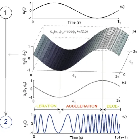
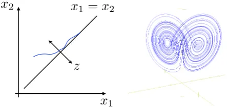
Figure 3 (color online). Schematic illustration of a phase dy-namics coupling function. The first oscillator x1 influences the second oscillatorx2 unidirectionally, as indicated by the directional diagram on the left of the figure. (a) Amplitude signalx1(t) during one cycle of periodT1. (b) Coupling func-tionq2(φ1, φ2) in {φ1, φ2}space. (c)φ2-averaged projection of the coupling functionq2(φ1, φ2). (d) Amplitude signal of the second driven oscillatorx2(t), during one cycle of the first oscillator. FromStankovskiet al.(2015).
To present the basic physics underlying a coupling function in the phase domain, we consider an elementary example of two phase oscillators that are unidirectionally phase-coupled:
˙ φ1=ω1
˙
φ2=ω2+q2(φ1, φ2) =ω2+ cos(φ1+π/2.5).
(9)
Our aim is to describe the effect of the coupling function q2(φ1, φ2) through which the first oscillator influences the
second one. From the expression for ˙φ2in Eq. (9) one can
appreciate the fundamental role of the coupling function: q2(φ1, φ2) is added to the frequencyω2. Thuschanges in
the magnitude ofq2(φ1, φ2)will contribute to the overall
change of the frequency of the second oscillator. Hence, depending on the value of q2(φ1, φ2), the second
oscil-lator will either accelerate or decelerate relative to its uncoupled motion.
The description of the phase coupling function is illus-trated schematically in Fig. 3. Because in real situations one measures the amplitude state of signals, we explain how the amplitude signals (Fig. 3(a) and (d)) are af-fected depending on the specific phase coupling function (Fig. 3(b) and (c)). In all plots, time is scaled relative to the periodT1of the amplitude of the signal
[image:8.595.319.561.50.297.2]Figure 4 (color online). Two characteristic coupling functions in the phase domain. (a) The coupling function q(φ1, φ2) is of sinusoidal form for the phase difference, as used in the Kuramoto model. (b) The coupling function q(φ1, φ2) is a product of the influence and sensitivity functions, as used in the Winfree model.
For convenient visualisation of the effects we set the sec-ond oscillator to be fifteen times slower than the first oscillator: ω2/ω1 = 15. The particular coupling
func-tionq2(φ1, φ2) = cos(φ1+π/2.5) presented on a 2π×2π
grid (Fig. 3(b)) resembles a shifted cosine wave, which changes only along the φ1-axis, like a direct coupling
component. Because all the changes occur along theφ1
-axis, and for easier comparison, we also present in Fig. 3(c) aφ2-averaged projection ofq2(φ1, φ2).
Finally, Fig. 3(d) shows how the second oscillatorx2(t)
is affected by the first oscillator in time in relation to the phase of the coupling function: when the coupling function q2(φ1, φ2) is increasing, the second oscillator
x2(t) accelerates; similarly, when q2(φ1, φ2) decreases,
x2(t) decelerates. Thus the form of the coupling
func-tion q2(φ1, φ2) shows in detail the mechanism through
which the dynamics and the oscillations of the second oscillator are affected: in this case they were alternately accelerated or decelerated by the influence of the first oscillator.
Of course, coupling functions can in general be much more complex than the simple example presented (cos(φ1+π/2.5)). This form of phase coupling function
with a direct contribution (predominantly) only from the other oscillator is often found as a coupling component in real applications, as will be discussed below. Other characteristic phase coupling functions of that kind could include the coupling functions from the Kuramoto model (Eq. (8)) and the Winfree model (Eq. (7)), as shown in Fig. 4. The sinusoidal function of the phase difference from the Kuramoto model exhibits a diagonal form in Fig. 4(a), while the influence-sensitivity product func-tion of Winfree model is given by a more complex form spread differently along the two-dimensional space in Fig. 4(b). Although these two functions differ from those in the previous example (Fig. 3), the procedure used for their interpretation is the same.
2. Amplitude coupling functions
Arguably, it is more natural to study amplitude dy-namics than phase dydy-namics, as the former is directly observable while the phase needs to be derived. Real systems often suffer from the “curse of dimensionality” (Keogh and Mueen,2011) in that not all of the features of a possible (hidden) higher-dimensional space are nec-essarily observable through the low-dimensional space of the measurements. Frequently, a delay embedding the-orem (Takens, 1981) is used to reconstruct the multi-dimensional dynamical system from data. In real appli-cation with non-autonomous and non-stationary dynam-ics, however the theorem often does not give the desired result (Clemson and Stefanovska, 2014). Nevertheless, amplitude state interactions also have a wide range of applications both in theory and methods, especially in the cases of chaotic systems, strong couplings, delayed systems, and large nonlinearities, including cases where complete synchronization (Cuomo and Oppenheim,1993;
Kocarev and Parlitz, 1995; Stankovski et al., 2014) and generalized synchronization(Abarbanelet al.,1993; Arn-holdet al.,1999;Kocarev and Parlitz,1996;Rulkovet al.,
1995; Stam et al., 2002) has been assessed through ob-servation of amplitude state space variables.
Amplitude coupling functions affect the interacting dy-namics by increasing or decreasing the state variables. Thus amplitude connectivity is defined by the connection and influence between the amplitude dynamics of the sys-tems. The form of the amplitude coupling function can often be a polynomial function or diffusive difference be-tween the states.
To present the basics of amplitude coupling functions, we discuss a simple example of two interacting Poincar´e limit-cycle oscillators. In the autonomous case, each of them is given by the polar (radialr and angular φ) co-ordinates as: ˙r = r(1−r) and ˙φ = ω. In this way, a Poincar´e oscillator is given by a circular limit-cycle and monotonically growing (isochronous) phase defined by the frequency parameter. In our example, we transform the polar variables to Cartesian (state space) coordinates x=rcos(φ),y=rsin(φ), and we set unidirectional cou-pling, such that the first (autonomous) oscillator:
˙
x1= 1− q
x2 1+y21
x1−ω1y1,
˙
y1= 1− q
x2 1+y21
y1+ω1x1,
(10)
is influencing thex2state of the second oscillator through
the quadratic coupling functionq2(x1, y1, x2, y2) =x21:
˙
x2= 1− q
x2 2+y22
x2−ω2y2+εx21,
˙
y2= 1− q
x2 2+y22
y2+ω2x2.
(11)
For simpler visual presentation we choose the first oscil-lator to be twenty times faster than the second one, i.e. their frequencies are in the ratioω2/ω1= 20, and we set
Figure 5 (color online). Schematic illustration of an ampli-tude dynamics coupling function. The first oscillator Eqs. (10) is influencing the second oscillator Eqs. (11) unidirec-tionally, as indicated by the directional diagram on the left of the figure. (a) Amplitude state signalx1(t) during one cycle of periodT1. (b) Coupling functionq2(x1, x2) in{x1, x2}space during one period of each of the oscillations. (c)x2-averaged projection of the coupling functionq2(x1, x2). (d) Amplitude signal of the second (driven) oscillatorx2(t), during one cycle of the first oscillator.
The description of the amplitude coupling function is illustrated schematically in Fig. 5. In theory, the cou-pling functionq2(x1, y1, x2, y2) has four variables, but for
better visual illustration, and because the dependence is only onx1, we show it only in respect to the two variables
x1andx2i.e.q2(x1, x2). The form of the coupling
func-tion is quadratic, and it changes only along thex1-axis, as
shown in Figs. 5(b) and (c). Finally, Fig. 5(d) shows how the second oscillatorx2(t) is affected by the first
oscilla-tor in time via the coupling function: when the quadratic coupling functionq2(x1, x2) is increasing, the amplitude
of the second oscillator x2(t) increases; similarly, when
q2(x1, x2) decreases,x2(t) decreases as well.
The particular example chosen for presentation used a quadratic functionx21; other examples include a direct linear coupling function e.g. x1, or a diffusive coupling
e.g. x2−x1 (Aronsonet al.,1990; Kocarev and Parlitz, 1996; Mirollo and Strogatz, 1990). There are a num-ber of methods which have inferred models that include amplitude coupling functions inherently (Friston, 2002;
Smelyanskiyet al.,2005; Voss et al., 2004) or have pre-estimated most probable models (Berger and Pericchi,
1996), but without including explicit assessment of the coupling functions. Due to the multi-dimensionality and the lack of a general property in a dynamical system (like for example the periodicity in phase dynamics), there are countless possibilities for generalization of the coupling
function. In a sense, this lack of general models is a de-ficiency in relation to the wider treatment of amplitude coupling functions. There are open questions here and much room for further work on generalising such models, in terms both of theory and methods, taking into account the amplitude properties of subgroups of dynamical sys-tems, including for example the chaotic, oscillatory, or reaction-diffusion nature of the systems.
3. Multivariate coupling functions
Thus far, we have been discussing pairwise coupling functions between two systems. In general, when inter-actions occur between more than two dynamical systems, in a network (Sec. III.D), there may be multivariate cou-pling functions with more than two input variables. For example, a multivariate phase coupling function could beq1(φ1, φ2, φ3), which is a triplet function of influence
in the dynamics of the first phase oscillator caused by a common dependence on three other phase oscillators. Such joint functional dependences can appear as clusters of subnetworks within a network (Albert and Barab´asi,
2002).
Multivariate interactions have been the subject of much attention recently, especially in developing meth-ods for detecting the couplings (Baselli et al., 1997;
Duggento et al., 2012; Faes et al., 2011; Frenzel and Pompe, 2007; Kralemann et al., 2011; Nawrath et al.,
2010; Paluˇs and Vejmelka, 2007). This is particularly relevant in networks, where one can miss part of the in-teractions if only pairwise links are inferred, or a spurious pairwise link can be inferred as being independent when they are actually part of a multivariate joint function. In terms of networks and graph theory, the multivariate coupling functions relate tohypergraph, which is defined as a generalization of a graph where an edge (or con-nection) can connect any number of nodes (or vertices) (Karypis and Kumar,2000;Weighill and Jacobson,2015;
Zass and Shashua,2008).
Multivariate coupling functions have been studied by inference of small-scale networks where the structural coupling can differ from the inferred effective coupling (Kralemann et al.,2011). The authors considered a net-work of three van der Pol oscillators where, in addition to pairwise couplings, there was also a joint multivariate cross-coupling function, for example of the formεx2x3in
the dynamics of the first oscillator ¨x1. Due to the
[image:10.595.56.298.49.280.2]Figure 6 (color online). Inference of multivari-ate interactions. True (structural) configura-tions (left), and the reconstructed phase model (right). Middle: the table shows the correspond-ing inferred couplcorrespond-ing strengths. Note the multi-variate triplet link – the arrows from the centres of the diagrams. FromKralemannet al.(2011).
– whereas in reality it is just an indirect effect from the actual joint multivariate coupling. In this way, the in-ference of multivariate coupling functions can provide a deeper insight into the connections in the network.
A corollary is the detection of triplet synchronization (Jia et al., 2015; Kralemann et al., 2013b). This is a synchronization phenomenon which has an explicit mul-tivariate coupling function of the formq1(φ1, φ2, φ3) and
which is tested in respect of the condition|mφ1+nφ2+
lφ3| ≤const, forn, m, l negative or positive. It is shown that the state of triplet synchronization can exist, even though each pair of systems remains asynchronous.
The brain mediates many oscillations and interactions on different levels (Park and Friston, 2013). Interac-tions between oscillaInterac-tions in different frequency bands are referred to as cross-frequency coupling in neuro-science (Jensen and Colgin, 2007). Recently, neural cross-frequency coupling functions were extracted from multivariate networks (Stankovski et al.,2015) (see also Sec. V.C). The network interactions between the five brainwave oscillationsδ,θ,α,β andγ were analysed by reconstruction of the multivariate phase dynamics, in-cluding the inference of triplet and quadruplet coupling functions. Fig. 7 shows a triplet coupling function of how theθ and αinfluence γ brain oscillations. It was found that the influence from theta oscillations is greater than from alpha, and that there is significant acceleration of gamma oscillations when the theta phase cycle changes fromπto 2π.
Very recently, Bicket al.(2016) have shown
theoreti-Figure 7 (color online). Multivariate triplet coupling tions between neural oscillations. The phase coupling func-tionqγ(φθ, φα) shows the influence thatθandαjointly insert on theγ cortical oscillations. FromStankovskiet al.(2015).
cally that symmetrically-coupled phase oscillators with multivariate (or non-pairwise) coupling functions can yield rich dynamics, including the emergence of chaos. This was observed even for as few asN= 4 oscillators. In contrast to the Kuramoto-Sakaguchi equations, the addi-tional multivariate coupling functions mean that one can find attracting chaos for a range of normal-form parame-ter values. Similarly, it was found that even the standard Kuramoto model can be chaotic with a finite number of oscillators (Popovych et al.,2005).
4. Generality of coupling functions
The coupling function is well-defined from a theoretical perspective. That is, once we have the model (as in Eqs. 1), the coupling function is unique and fixed. The solu-tions of the equasolu-tions also depend continuously on the coupling function. Small changes in the coupling func-tion will cause only small changes in the solufunc-tions over finite time intervals. If solutions are attracted to some set exponentially and uniformly fast, then small changes in the coupling do not affect the stability of the system. When we want to infer the coupling function from data we can face a number of challenges in obtaining a unique result (Sec. IV). Typically, we measure only projections of the coupling function, which might in it-self lead to non-uniqueness of the estimate. That is, we project the function (which is infinite-dimensional) onto a finite-dimensional vector space. In doing so, we could lose some information and, generically, it is not possible to estimate the function uniquely (even without taking account of noise and perturbations). Furthermore, the final form of the estimated function will depend on the choice and number of base functions. For example, the choice of Fourier series or general orthogonal polynomi-als as base functions can affect slightly the final estimate of the coupling function. The choice of which base func-tions to be used is infinite. Even though many aspects of coupling functions (like the number of arguments, decom-position under an appropriate model, analysis of coupling function components, prediction with coupling functions, etc.), can be applied with great generality, the coupling functions themselves cannot be determined uniquely.
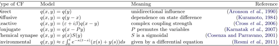
[image:11.595.73.281.520.671.2]Type of CF Model Meaning Reference Direct q(x, y) =q(y) unidirectional influence (Aronsonet al.,1990) Diffusive q(x, y) =q(y−x) dependence on state difference (Kuramoto,1984) Reactive q(x, y) = (ε+iβ)q(x−y) complex coupling strength (Crosset al.,2006) Conjugate q(x, y) =q(x−P y) P permutes the variables (Karnataket al.,2007) Chemical synapse q(x, y) =g(x)S(y) S is a sigmoidal (Cosenza and Parravano,2001) Environmental q(x, y)≈εRt
0e
−κ(t−s)(x(s) +y(s))ds given by a differential equation (Resmiet al.,2011) Table I Different examples of coupling functionsq. These pairwise coupling functions (CFs) are considered in relation to the system: ˙x=f(x) +q(x, y).
and the dynamics. Also in the literature, a diffusive coupling function q(y−x) satisfying a local condition q0(0) <0 is called dissipative coupling (Rul’Kov et al.,
1992). This condition resembles Fick’s law as the cou-pling forces the coupled system to converge towards the same state. Whenq0(0)>0 the coupling is called repul-sive (Henset al.,2013). Chemical synapses are an impor-tant form of coupling where the influences ofxandy ap-pear together as a product. There are also other interest-ing forms of couplinterest-ing such as the geometric mean and fur-ther generalizations (Petereit and Pikovsky,2017;Prasad et al.,2010). In environmental coupling, the function is given by the solution of a differential equation. In this case one can consider ˙y=−κy+ε(x(t) +y(t)) forκ >0, so that the variables are considered as external fields driv-ing the equation. Its solutiony(t) =y(t;x, y) is taken as the coupling function q(x, y) and, for t 1, is given in the table. The generality of coupling functions, and the fact that the form can come from an unbounded set of functions, were used to construct the encryption key in a secure communications protocol (Stankovskiet al.,2014) (see Sec. V.F).
D. Coupling functions revealing mechanisms
The functional form is a qualitative property that de-fines the mechanism and acts as an additional dimension to complement the quantitative characteristics such as the coupling strength, directionality, frequency param-eter and limit-cycle shape paramparam-eters. By definition, the mechanism involves some kind of function or process leading to a change in the affected system. Its signifi-cance is that it may lead to qualitative transitions and induce or reduce physical effects, including synchroniza-tion, instability, amplitude death, or oscillation death.
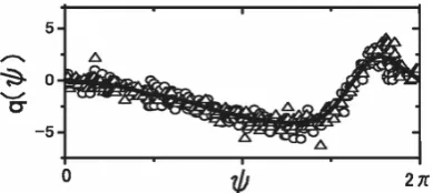
But why is the mechanism important, and how it can be used? The first and foremost use of the coupling func-tion mechanism is to illuminate the nature of the interac-tions themselves. For example, the coupling function of the Belousov-Zhabotinsky chemical oscillator has been reconstructed (Miyazaki and Kinoshita, 2006) with the help of a method for the inference of phase dynamics. Fig. 8 shows such a coupling function, demonstrating a form that is very far from a sinusoidal function: a curve that gradually decreases in the region of a smallψ and abruptly increases at a larger ψ, with its minimum and
maximum at around 5/4πand 7/4π, respectively. Another important set of examples is the class of cou-pling functions and phase response curves used in neu-roscience. In neuronal interactions, some variables are very spike-like i.e. they resemble delta functions. Con-sequently, neuronal coupling functions (which are con-volution of phase response curves and perturbation func-tions) then depend only, or mainly, on the phase response curves. So the interaction mechanism is defined by the phase response curves: quite a lot of work has been done in this direction (Ermentrout,1996;Gouwenset al.,2010;
Schultheisset al.,2011;Tateno and Robinson,2007); see also Sec. IV.D.2. For example, Tateno and Robinson
(2007) and Gouwens et al. (2010) reconstructed experi-mentally the phase response curves for different types of interneurons in rat cortex, in order to better understand the mechanisms of neural synchronization.
The mechanism of a coupling function depends on the differing contributions from individual oscillators. Changes in form may depend predominantly on only one of the phases (along one-axis), or they may depend on both phases, often resulting in a complicated and intuitively unclear dependance. The mechanism speci-fied by the form of the coupling function can be used to distinguish the individual functional contributions to a coupling. One can decompose the net coupling func-tion into components describing the self, direct and indi-rect couplings (Iatsenko et al., 2013). The self-coupling describes the inner dynamics of an oscillator which re-sults from the interactions and has little physical mean-ing. Direct-coupling describes the influence of the di-rect (unididi-rectional) driving that one oscillator exerts on the other. The last component, indirect-coupling, often called common-coupling, depends on the shared contri-butions of the two oscillators e.g. the diffusive coupling given with the phase difference terms. This functional coupling decomposition can be further generalized for multivariate coupling functions, where for example, a di-rect coupling from two oscillators to a third one can be determined (Stankovski et al.,2015).
[image:12.595.69.555.50.131.2]Figure 8 Coupling function determined from the phase dy-namics of two interacting chemical Belousov-Zhabotinsky os-cillators. The coupling function is reconstructed in terms of the phase difference ψ=φ2−φ1. Points obtained from re-actors 1 and 2 are plotted with open circles and triangles, respectively. The full curves represent smooth interpolations. FromMiyazaki and Kinoshita(2006).
Furthermore, the mechanisms and form of the coupling functions can be used to engineer and construct a partic-ular complex dynamical structure, including sequential patterns and desynchronization of electrochemical oscil-lations (Kisset al., 2007). Even more importantly, one can use knowledge about the mechanism of the recon-structed coupling function to predict transitions of the physical effects – an important property described in de-tail for synchronization in the following section.
E. Synchronization prediction with coupling functions
Synchronization is a widespread phenomenon whose occurrence and disappearance can be of great impor-tance. For example, epileptic seizures in the brain are associated with excessive synchronization between a large number of neurons, so there is a need to control synchro-nization to provide a means of stopping or preventing seizures (Schindleret al.,2007); while in power grids the maintenance of synchronization is of crucial importance (Rubido, 2015). Therefore, one often needs to be able to control and predict the onset and disappearance of synchronization.
A seminal work on coupling functions by Kiss et al.
(2005) uses the inferred knowledge of thecoupling func-tion to predictcharacteristic synchronization phenomena in electrochemical oscillators. In particular, the authors demonstrated the power of phase coupling functions, ob-tained from direct experiments on a single oscillator, to predict the dependence of synchronization characteristics such as order-disorder transitions on system parameters, both in small sets and in large populations of interacting electrochemical oscillators.
The authors investigated the parametric dependence of mutual entrainment using an electrochemical reaction system, the electrodissolution of nickel in sulfuric acid (see also Sec. V.A for further applications on chemical coupling functions). A single nickel electrodissolution oscillator can have two main characteristic waveforms of periodic oscillation – the smooth type and the relax-ation oscillrelax-ation type. The phase response curve is of the
(a)
(b)
(c)
Figure 9 Experimental coupling function from electrochemi-cal oscillators, used for the prediction of synchronization. (a)-(c) Coupling functionq(ψ) evaluated in respect of the phase differenceψ =φ2−φ1 shown on the left panel and its odd part q−(∆φ) shown on the right panel – for the case of (a) smooth oscillator, and (b) and (c) for relaxation oscillator with slightly different parameters. H(∆φ) on the plots is equivalent to the q(ψ) notation used in the current review. FromKisset al.(2005).
smooth type and is nearly sinusoidal, while being more asymmetric for the relaxation oscillations.
The coupling functions are calculated using the phase response curve obtained from experimental data for the variable through which the oscillators are coupled. The coupling functionsq(ψ) of two coupled oscillators are re-constructed for three characteristic cases, as shown in Fig. 9(a)-(c), left panels. The right panels in Fig. 9 show the corresponding odd (antisymmetric) part of the cou-pling functionsq−(ψ) = [q(ψ)−q(−ψ)]/2, which is im-portant for determination of the synchronization. The coupling functionsq(ψ) Fig. 9 (a)-(c) have predominantly positive values, so the interactions contribute to the ac-celeration of the affected oscillators. The first coupling function Fig. 9(a) for smooth oscillations has a sinu-soidalq−(ψ) which can lead to in-phase synchronization at the phase difference ofψ∗ = 0. The third case of re-laxation oscillations Fig. 9(c) has an inverted sinusoidal formq−(ψ), leading to stable anti-phase synchronization at ψ∗ = π. The most peculiar case is the second one Fig. 9(b) of relaxation oscillations, where the odd cou-pling functionq−(ψ) takes the form of a second harmonic (q−(ψ) ≈sin(2ψ)) and both the in-phase (ψ∗ = 0) and anti-phase (ψ∗ = π) entrainments are stable, in which case the actual state attained will depend on the initial conditions.
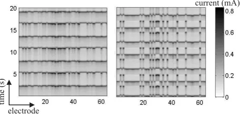
[image:13.595.325.551.59.279.2]ti
me
(s
)
electrode
current (mA)
Figure 10 Mutual entrainment and stable single-cluster (left panel) and two-cluster (right panel) states of a population of 64globally-coupled electrochemical relaxation oscillators un-der the same experimental conditions. The two-cluster state was obtained from the one-cluster state by a small perturba-tion acting as a different initial condiperturba-tion for the populaperturba-tion. FromKisset al.(2005).
a single oscillator was applied to predict the onset of syn-chronization in experiments with 64 globally coupled cillators. The experiments confirmed that for smooth os-cillators the interactions converge to a single cluster, and for relaxational oscillators they converge to a two-cluster synchronized state. Experiments in a parameter region between these states, in which bistability is predicted, are shown in Fig. 10. A small perturbation of the stable one-cluster state (left panel of Fig. 10) yields a stable two-cluster state (right panel of Fig. 10). Therefore, all the synchronization behavior seen in the experiments was in agreement with prior predictions based on the coupling functions.
In a separate line of work, synchronization was also predicted in neuroscience: interaction mechanisms in-volving individual neurons, usually in terms of phase-response curves (PRCs) or spike-time phase-response-curves (STRCs), were used to understand and predict the syn-chronous behavior of networks of neurons (Acker et al.,
2003; Netoff et al., 2005; Schultheiss et al., 2011). For example,Netoffet al.(2005) studied experimentally the spike-time response-curves of individual neuronal cells. Results from these single-cell experiments were then used to predict the multi-cell network behaviors, which were found to be compatible with previous model-based pre-dictions of how specific membrane mechanisms give rise to the empirically measured synchronization behavior.
F. Unifying nomenclature
Over the course of time, physicists have used a range of different terminology for coupling functions. For exam-ple, some publications refer to them as interaction func-tions and some as coupling funcfunc-tions. This inconsistency needs to be overcome by adopting a common nomencla-ture for the funomencla-ture.
The terms interaction function and coupling function have both been used to describe the physical and
mathe-matical links between interacting dynamical systems. Of these, coupling function has been used about twice as of-ten in the literature, including the most recent. The term coupling is closer to describing a connection between two systems, while the term interaction is more general. Cou-pling implies causality, whereas interaction does not nec-essarily do so. Often correlation and coherence are con-sidered as signatures of interactions, while they do not necessarily imply the existence of couplings. We therefore propose that the terminology be unified, and the term coupling function be used henceforth to characterise the link between two dynamical systems whose interaction is also causal.
III. THEORY
In physics one is likely to examine stable static config-urations whereas, in dynamical interaction between os-cillators, solutions will converge to a subspace. For ex-ample, if two oscillators are in complete synchronization the subspace is called thesynchronization manifold and corresponds to the case where the oscillators are in the same state for all time (Fujisaka and Yamada,1983; Pec-ora and Carroll,1990). So, within the subspace, the os-cillators have their own dynamics and finer information on the coupling function is needed.
The analytical techniques and methods needed to an-alyze the dynamics will depend on whether the coupling strength is strong or weak. Roughly speaking, in the strong coupling regime, we will have to tackle the fully-coupled oscillators whereas in the weak coupling we can reduce the analysis to lower-dimensional equations.
A. Strong interaction
To illustrate the main ideas and challenges of treating the case of strong interaction, while keeping technicalities to a minimum, we will first discuss the case of two coupled oscillators. These examples contain the main ideas and reveal the role of the coupling function and how it guides the system towards synchronization.
1. Two coupled oscillators
We start by illustrating the variety of dynamical phe-nomena that can be encountered and the role played by the coupling function in the strong coupling regime.
Diffusion driven oscillations
[image:14.595.61.297.58.172.2]oscillate when diffusively coupled. This phenomenon is calleddiffusion driven oscillation.
Assume that the system
˙
x=f(x), (12)
where f : Rn →
Rn is a differentiable vector field with
a globally stable attraction with point – all trajectories will converge to this point. Now consider two of such systems coupled diffusively
˙
x1 = f(x1) +εH(x2−x1) (13)
˙
x2 = f(x2) +εH(x1−x2).
The problem proposed by Smale was to find (if possible) a coupling function (positive definite matrix)Hsuch that the diffusively coupled system undergoes a Hopf bifurca-tion. Loosely speaking, one may think of two cells that by themselves are inert but which, when they interact diffusively, become alive in a dynamical sense and start to oscillate.
Interestingly, the dimension of the uncoupled systems comes into play. Smale constructed an example in four di-mensions. Pogromskyet al.(1999) constructed examples in three dimensions and also showed that, under suitable conditions, the minimum dimension for diffusive coupling to result in oscillation is n= 3. The following example illustrates the main ideas. Consider
f(x) =Ax(1 +|x|2) withA=
1 −1 1
1 0 0
−4 2 −3
, (14)
where |x|2 = xTx. Note that all the eigenvalues of A have negative real parts. So the origin of the system Eq. (14) is exponentially attracting.
Consider the coupling function to be the identity
˙
x1=f(x1) +ε(x2−x1)
˙
x2=f(x2) +ε(x1−x2).
For ε = 0 the origin is globally attracting; the uniform attraction persists whenε is very small, and so the ori-gin is still globally attracting. However, for large values of the coupling ε > 0.6512 the coupled systems exhibit oscillatory solutions (the origin has undergone a Hopf bi-furcation).
Generalizations: In this example the coupling func-tion was the identity. Pogromsky et al.(1999) discussed further coupling functions, such as coupling functions of rank two that generate diffusion-driven oscillators. Fur-ther oscillations in originally passive systems have been reported in spatially extended systems (Gomez-Marin et al.,2007). In diffusively coupled membranes, collective oscillation in a group of nonoscillatory cells can also occur as a result of spatially inhomogeneous activation factor (Ma and Yoshikawa,2009). These ideas of diffusion lead-ing to chemical differentiation have also been observed experimentally and generalized by including heterogene-ity in the model (Tompkinset al.,2014).
Oscillation death
We now consider the opposite problem: Systems which when isolated exhibit oscillatory behaviour but which, when coupled diffusively, cease to oscillate and where the solutions converge to an equilibrium point.
As mentioned above in Sec. IB, this phenomenon is calledoscillation death (Bar-Eli,1985;Ermentrout and Kopell,1990;Koseskaet al.,2013a;Mirollo and Strogatz,
1990). To illustrate the essential features we consider a normal form of the Hopf bifurcation
˙
xj =fj(xj)
where
fj(x) =ωjAx+ (1− |x|2)x, withA=
0 −1 1 0
.
So, each isolated system has a limit cycle of amplitude
|x|2= 1 and a frequency ofω
j. Note that the originx= 0 is an unstable equilibrium point. In oscillation death when the systems are coupled, the origin may become stable.
Focusing on diffusive coupling, again, the question con-cerns the nature of the coupling function. Aronsonet al.
(1990) remarked that the simplest coupling function to have the desired properties is the identity with strength ε. The equations have the same form as Eq. (13) with H being the identity.
The effect can be better understood in terms of phase and amplitude variables. Let r1, r2 be the amplitudes
and φ1, φ2 the phases of x1 and x2, respectively. We
consider r1 = r2 = r which captures the main causes
of the effect, as well as the phase difference ψ = φ1−
φ2. Then the equations in these variables can be well
approximated as
˙
r = r(1−ε−r2) +εrcosψ (15)
˙
ψ = ∆ω−2εsinψ. (16)
The conditions for oscillation death are a stable fixed point at r = 0 along with a stable fixed point for the phase dynamics. The above equations provide the main mechanism for oscillation death. First, we can deter-mine the stable fixed point for the phase dynamics, as il-lustrated in Fig. 2. There is a fixed pointψ∗ifε >∆
ω/2 and sinψ∗ = ∆ω/(2ε). We will assume that ∆ω > 2 which implies that, when the fixed pointψ∗exists,ε >1. Next, we analyse the stability of the fixed pointr∗= 0. This is determined by the linear part of Eq. 15. Hence, the condition for stability is
1−ε+εcosψ∗<0.
Using the equation for the fixed point we have cosψ∗ =
p