Noname manuscript No.
(will be inserted by the editor)
Fast separation for the three-index assignment problem
Trivikram Dokka · Ioannis Mourtos · Frits C.R. Spieksma
Received: date / Accepted: date
Abstract A critical step in a cutting plane algorithm is separation, i.e., establishing whether a given vector x violates an inequality belonging to a specific class. It is customary to express the time complexity of a separation algorithm in the number of variablesn. Here, we argue that a separation algorithm may instead process the vector containing the positive components ofx,denoted assupp(x),which offers a more compact representation, especially ifxis sparse; we also propose to express the time complexity in terms of|supp(x)|.Although several well-known separation algorithms exploit the sparsity ofx,we revisit this idea in order to take sparsity explicitly into account in the time-complexity of separation and also design faster algorithms. We apply this approach to two classes of facet-defining inequalities for the three-index assignment problem, and obtain separation algorithms whose time complexity is linear in |supp(x)| instead of n.We indicate that this can be generalized to the axial k -index assignment problem and we show empirically how the separation algorithms exploiting sparsity improve on existing ones by running them on the largest instances reported in the literature.
This paper is an improved version of an extended abstract that appeared as “Fast separation algorithms for three index assignment problems” in the proceedings of ISCO 2012, LNCS 7422, pp. 189-200, 2012. This research has been co-financed by the European Union (European Social Fund ESF) and Greek national funds through the Operational Program Education and Lifelong Learning of the National Strategic Refer-ence Framework (NSRF) - Research Funding Program: Thales: Investing in knowledge society through the European Social Fund (MIS: 380232), and this research has been supported by the Interuniversity Attraction Poles Programme initiated by the Belgian Science Policy.
Trivikram Dokka
Department of Management Science, Lancaster University Management School,Lancaster, LA1 14X, United Kingdom.
E-mail: [email protected]
Ioannis Mourtos
Department of Management Science and Technology, Athens University of Economics and Business, 76 Patission Ave. 1043 34 Athens, Greece.
E-mail: [email protected]
Frits C.R. Spieksma
1 Motivation
Cutting plane algorithms constitute a fundamental way of solving combinatorial optimiza-tion problems. Typically, in such an approach, a specific combinatorial optimizaoptimiza-tion problem is formulated as an Integer Linear Program (ILP) of the form min{cTx: Ax=b, x∈Zn
+}, wherexdenotes ann-dimensional column vector of variables andA, b,andcare matrices of appropriate dimension. The convex hull of the feasible solutions is defined by the correspond-ing polyhedronPI = conv{x∈Z+n :Ax=b}. Then, there is interest in identifying classes of inequalities that are valid forPI and, preferably, facet-defining (for related background see, for example, [23]). Although identifying such families provides a (partial) characterization of
PI, the computational benefit of these families, in terms of findingz= min{cTx:x∈PI}, can be realized only if these inequalities can efficiently be added to the linear programming (LP) relaxationPL= min{cTx: Ax=b, x≥0}.
Since there can be many inequalities within a family, their addition within a cutting plane scheme should be made ‘on demand’, i.e., an inequality should added to the current LP-relaxation only if violated by a specific vector x ∈ Rn. The problem of determining whether such a vector violates an inequality of a specific family is called the separation
problem for this family and an algorithm solving it is called a separation algorithm. Hence
the importance of designing, typically family-specific, separation algorithms that should be of low computational complexity.
It is quite customary to express the complexity of a separation algorithm in terms ofn, the dimension of the vectorx. This seems reasonable since, at the very least, one would need to inspect every entry of the vectorxto decide whether a violated inequality exists. In fact, separation algorithms with a complexity ofO(n) have been called “best-possible” for the 3-index assignment problem [4, 21]. If the input to a separation algorithm is an optimal solution to the current LP-relaxation, i.e., a vector x∈PL\PI, such an input is typicallysparse in the sense that few entries ofxare positive. Thus, replacingxby its support supp(x) offers a more compact representation of the input. This leads to the following question: when the input to a separation algorithm is supp(x), is it possible to obtain faster separation algorithms and express their time-complexity in terms of|supp(x)|?
Clearly, the input to a separation algorithm cannot be restricted to x-vectors that rep-resent extreme vertices of the LP-relaxation at hand. Indeed, any x-vector is a potential input to the separation algorithm. For example, one might be interested in separating vec-tors that do not represent vertices, because the solution of the LP-relaxation is obtained via an interior point method, or because the vector to be separated is a vertex from a differ-ent relaxation. We point out that our results hold in such cases as well, since any vector x
can be encoded by listing the|supp(x)| positive components ofx. However, it is true that the advantage of this more compact input in terms of algorithm’s running time disappears. Thus, representing a vector xby using the support leads to speedups when the vector is sparse. This typically happens when a separation algorithm is incorporated within aBranch
& Cut or a cutting plane scheme, since then the separation algorithm receives as input not
anyx∈Rn, but a vertexx∈PL\P
I, which is sparse particularly for problems having much more variables than constraints.
separation in terms ofsupp(x) is plausible (Section 5). That is, we obtain algorithms of time
O(|supp(x)|), which are much faster than existing ones ofO(n) time [4] for separating not only vertices of the LP-relaxation but any sparse vector; the algorithms of [4] neither exploit sparsity nor assume that the input vector is a vertex. We also propose such algorithms for thek-index assignment problem (Section 6). Testing the performance of our separation algorithms on large literature instances for the 3-index assignment problem offers strong empirical support for our effort (Section 7).
2 Exploiting sparsity in separation algorithms
Traditionally, to describe the input needed for an algorithm separating a specific class of inequalities, then entries of the vectorx= (x1, . . . , xn) are provided. We propose here an alternative measure of the input: the cardinality of the support of the vectorx, denoted by
T =|supp(x)|. That is, we propose to express the running time of a separation algorithm in terms ofT.This allows us to exploit the fact that the input received by a separation algorithm is not any vectorxbut, typically in cutting plane schemes, the vertex of a polyhedron having several zero entries.
It could be of help to consider the following (imaginary) setting. Suppose that several instances of some combinatorial optimization problem are being solved in parallel through a cutting-plane approach, using multiple computers. However, only a single computer is available for the separation routine. Then, this routine receives several fractional vectors corresponding to the instances being solved by the cutting-plane approach. In such a sit-uation, one easily imagines that the sole input to the separation routine are the positive components of the vectorx, i.e.,supp(x).In other words, we examine the decision problem with respect to a certain class of valid inequalitiesC, as follows:
– INPUT:support(x)
– QUESTION: Is there an inequality violated byxinC?
Let us emphasize that this idea is not new, since there are many examples in the literature where sparsity is implicitly used in the design of separation algorithms. The oldest such example concerns the traveling salesman problem (TSP) and the well-known class of subtour elimination constraints [3]. Assuming a binary variablexe per edgee, these inequalities are formulated as
X
e:|e∩S|= 1
xe≥2 for any nonempty proper subsetS of cities.
Another indicative case is the separation ofodd-cycleinequalities for the stable set prob-lem. If ˜C is the set of all induced odd cycles in the underlying graph, such an inequality is
X
e∈C
xe≤
|C| −1
2 for eachC∈ ˜
C. (1)
To separate odd-cycle inequalities for a given vector x∗, shortest paths are computed in an bipartite graph H [23, p.1186-1187]). The complexity of this separation algorithm is
O(|V| · |E| ·log|V|) [10, 9], although zero-weighted edges may result in nodes and edges ofH
not required in the shortest path calculation [22].
Regarding the index selection problem, formulated as a set packing problem [8], the separation of lifted odd-hole inequalities is accomplished by determining a minimum-weight odd cycle in a graph having one node for each fractional variable, where the weight of each edge depends only on the positive components ofx∗. The number of variables is much larger than the number of constraint, thus anyx∗ produced by the LP-relaxation is sparse because the number of its positive components is bounded by the number of constraints.
Further examples of separation procedures that use only the fractional components of the solution to the LP-relaxation have been proposed for the 0−1 knapsack problem [16], the winner determination problem in combinatorial auctions [18], the sequence alignment problem [17], the time-indexed formulation of single-machine scheduling [12] and the pallet loading problem [1].
Overall, it is common that separation algorithms receive as input a vertex of the LP-relaxation and that such a vector is sparse, particularly when the number of variables is larger than the number of constraints.
3 The 3-index assignment polytope (3AP)
The 3-index assignment problem, defined on three disjointn-setsI, J, K and a weight func-tion w: I×J×K −→ R, asks for a collection of triples M ⊆I×J ×K such that each
element of each set appears in exactly one triple, and the functionwis minimized (over all possible such collections). Its formulation as an integer linear program is
min P
i∈I
P
j∈J
P
k∈K
wijkxijk
s.t. P
j∈J
P
k∈K
xijk= 1 ∀i∈I, (2)
P
i∈I
P
k∈K
xijk= 1 ∀j∈J, (3)
P
i∈I
P
j∈J
xijk= 1 ∀k∈K, (4)
xijk∈ {0,1} ∀i∈I, j∈J, k∈K. (5)
Let An denote the (0,1) matrix corresponding to the constraints (2) - (4), which has
n3 columns and 3nrows. Notice that hereafter n denotes the cardinality of each set being ‘assigned’, hence the number of variables is n3. Then, the 3-index assignment polytope is
PI = conv{x∈ {0,1}n 3
: Anx= e}, while its LP-relaxation is Pn = {x ∈ Rn3 : Anx =
The first investigation of the facial structure ofPI appears in [5]. Let us describe the two families of facet-defining inequalities presented in [5]. Thecolumn intersection graph ofAn,
namelyG(V, E), has a node for each column of An and an edge for every pair of columns that have a +1 entry in the same row. Notice that a column contains three +1’s. We define the intersection of two columnsc anddas the set of rows of An such that each row in the set has a +1 entry in columncand in columnd; this is denoted by|c∩d|. It is easy to see thatV =I×J×K andE={(c, d) :{c, d} ⊆V,|c∩d| ≥1},i.e., a node inV corresponds to a triple, and two nodes are connected if the corresponding triples share some index. A
clique is a maximal completesubgraph.
Clearly, a clique in G corresponds to a valid inequality with right-hand side 1. In fact,
G(V, E) contains two types of cliques, each yielding a family of inequalities that are facet-defining forPI. To formally define the two types of clique inequalities, let
– for eachc∈V :Q(c) ={d∈V :|c∩d| ≥2},
– for eachc∈V : coQ(c) ={d∈V :|c∩d|= 1}, and
– for eachc, d∈V with|c∩d|= 0 :Q(c, d) ={c} ∪ {Q(d)∩coQ(c)}.
Thus,Q(c) is the set of triples sharing at least two indices with triplec, while coQ(c) is the set of triples that has exactly one index in common with triple c. Finally, when given two disjoint triplescandd,Q(c, d) is the set of triples that has two indices in common with
d, and one withc, together with triplec. Notice thatQ(c, d) has exactly four elements. As usual, we writex(A) forP
q∈Axq.
Definition 1 For each c ∈ V, the facet-defining inequalityx(Q(c))≤1 is called a clique
inequality of type I.
Once we organize the variables xijk in a three-dimensional array (a cube), a clique inequality of type I can be seen as the sum of thosex-variables that lie on the three “axes” through a particular cell (see Figure 1 for a geometric illustration).
Definition 2 For eachc, d∈V with|c∩d|= 0, the facet-defining inequalityx(Q(c, d))≤1 is called aclique inequality of type II.
An illustration of a clique inequality of type II is given in Figure 2.
The separation of inequalities induced by cliques of type I and II was first treated in [5] through algorithms ofO(n4) time complexity. ImprovedO(n3) algorithms (i.e., of complexity linear in the number of variables) appear in Balas and Qi [4], in which they are characterized as “best-possible”. We illustrate them also here as Algorithms 1 and 2.
To discuss how improved separation algorithms can be obtained by using a compact input, let us recall from linear programming that the number of non-zero variables in a vertex of the LP-relaxation cannot exceed the number of constraints.
Remark 1 A solution corresponding to a vertex ofPn has at most 3nnon-zero variables.
Given a vector x∈ Pn, let supp(x) = {c ∈ V : x
c > 0} and T =|supp(x)|. To ease the presentation, let us assume that supp(x) contains the triples indexing the non-zero entries ofxand the corresponding (positive) fraction per triple.
I
K
J
(i,j,k)
Fig. 1 Geometric illustration of a clique inequality of type I; the three dotted axes correspond to the variables in this inequality
k
icjdkd idjdkd
icjckd idjcjd
j
icjdkc idjdkc
icjckc idjckc i
Fig. 2 Geometric illustration of a clique inequality of type II; the four highlighted cells correspond to the four variables in this inequality.
than the O(n3) time complexity of Algorithms 1 and 2; notice that O(T) reaches O(n3) only ifxis ‘fully dense’. Our algorithms achieve such a speed-up by pre-calculating certain sums ofx’s entries and, as expected, by utilising the fact that the input vector contains only non-zero values. Thus their main difference from Algorithms 1 and 2 is their effective use of sparsity.
4 Notation and preliminaries
[image:6.595.125.386.89.302.2] [image:6.595.175.350.366.458.2]Algorithm 1Balas & Qi Separation Algorithm for cliques of type I {Input: the vectorxand an integerv≥4}
for allc∈V do
dc:= 0;
end for for allc∈V do
ifxc≥v1·n then
for allt∈Q(c)do
dt:=dt+xc;
ifdt>1then
returnx(Q(t))≤1 as violated;
end if end for end if end for for allc∈V do
ifdc>v−33 then computex(Q(c));
ifx(Q(c))>1then
returnx(Q(c))≤1 as violated;
end if end if end for
Algorithm 2Balas & Qi Separation Algorithm for cliques of type II {Input: the vectorx}
for allc∈V :14< xc<1do
for allt∈V :|t∩c|= 1do ifxt> 1−3xc then
for alld∈V :|d∩c|= 0 and|d∩t|= 2do
computex(Q(c, d));
if x(Q(c, d))>1then
returnx(Q(c, d))≤1 as violated;
end if end for end if end for end for
to a set of ‘core’ elements C ⊂I∪J ∪K, in the sense that given C and supp(x) we can explicitly compute the left-hand side of the inequality. For example, each clique inequality of type I corresponds to a C having one element from each of I,J andK. Similarly, for a clique inequality of type II, the corresponding C contains two elements from each of I, J
andK. Therefore, a natural idea when searching for a violated inequality from a particular class is to identify the set C the inequality corresponds to. A naive algorithm would check all possible C’s; clearly, this can be prohibitively expensive as the cardinality of C and n
increases.
The algorithms presented here find the C of a violated inequality by exploiting the properties of a point inPn. To show these properties, we introduce some notation. Define, forx∈Pn:
– for eachj∈J, k∈K: SUMI(j, k) =P
i∈I
– for eachi∈I, k∈K: SUMJ(i, k) = P
j∈J
xijk,
– for eachi∈I, j∈J: SUMK(i, j) = P
k∈K
xijk.
Informally, each of these quantities corresponds to an axis in the geometric description given in Figure 1.
Lemma 1 Let >0. For all i∈I, the number of pairs(i, j)(respectively number of pairs
(i, k)),j ∈J (k∈K), such that SUMK(i, j)> (respectively SUMJ(i, k)> ) is at most
1 n.
Proof If not, at least 1npairs (i, j)∈I×J have SUMK(i, j)> . This implies we have
X
i
X
j
SUMK(i, j)> 1
·n=n=
X
i
X
j
X
k
xijk =
X
i
X
j
SUMK(i, j)
which is a contradiction. ut
Further, we define
– for eachi∈I:J(i) ={j∈J : SUMK(i, j)> 13}.
Notice that|J(i)| ≤2 for eachi∈I, due to (2) and Lemma 1.
We can compute all aforementioned quantities by scanning supp(x) only once. For ex-ample, to compute SUMI(j, k) for a specific j, k, it suffices to add the values of xv’s for each triplev ∈V having|v∩ {j, k}|= 2 encountered while scanningsupp(x). Algorithm 3 describes all steps in detail.
Algorithm 3Calculating SUMI(j, k) andJ(i) {Input:supp(x)}
for allc∈supp(x) withc= (ic, jc, kc)do
ifvariable SUMK(ic, jc) does not existthen create variable SUMK(ic, jc);
SUMK(ic, jc) := 0;
end if
SUMK(ic, jc) := SUMK(ic, jc) +xc;
ifSUMK(ic, jc)>13 then
ifJ(ic) does not existthen create variableJ(ic);
end if
J(ic) :=J(ic)∪ {jc};
end if end for
Lemma 2 For an arbitrary x∈Pn, all positive SUMI(j, k), SUMJ(i, k) and SUMK(i, j)
values (for i∈I, j ∈J, k ∈K) as well as the sets J(i)for each i∈I can be calculated in
O(T) steps.
Proof Algorithm 3 shows how to compute SUMI(j, k), for eachj, k, as well asJ(i) for each
For each i ∈I (resp j ∈J, k ∈ K), let val(i) (resp.val(j),val(k)) be the value of the third largest variable indexed by a triple containing i (resp.j, k). Then we define for any
x∈Pn:
– for eachi∈I:A(i) ={(i, j, k)∈V :xijk ≥val(i), j∈J, k∈K},
– for eachj∈J:B(j) ={(i, j, k)∈V :xijk≥val(j), i∈I, k∈K},
– for eachk∈K:C(k) ={(i, j, k)∈V :xijk≥val(k), i∈I, j∈J}.
It follows that the setsA(i) (resp.B(j), C(k)) contain the largest three such variables, i.e. the three largest variables indexed by a triple containingi(resp.j, k). In addition, we define
– for eachi∈I:A>1
4(i) ={(i, j, k)∈V : xijk> 1
4, j∈J, k∈K},
– for eachj∈J:B>1
4(j) ={(i, j, k)∈V : xijk> 1
4, i∈I, k∈K},
– for eachk∈K:C>14(k) ={(i, j, k)∈V : xijk> 1
4, i∈I, j∈J}.
Observe further that all elements from a specific A>1
4(i) (resp.B> 1
4(j), C> 1
4(k)) occur in a single equality among equalities (2) (resp. (3), (4)). Since the right-hand side of any equality is 1, and each element in any such set has value strictly larger than 14, it follows that |A>1
4(i)| ≤3,|B>14(j)| ≤3, and|C>14(k)| ≤3, fori∈I, j∈J, k∈K. In fact, we can state the following.
Lemma 3 For every fixed >0 andi ∈I, the number of triples (i, j, k), withj ∈J and
k∈K, such that xijk > is at most 1 −1.
Again, scanning supp(x) only once allows us to compute the sets defined above. That is, whenever we encounter a triplev∈V insupp(x) with|v∩i1|= 1, then ifxv>14 we addvto
A>1
4(i1) and ifxv is larger thanxuwithu∈A(i1) we replaceuwithvinA(i1). Algorithm 4 contains all related steps.
Lemma 4 For an arbitrary x∈Pn, the setsA(i) andA>1
4(i) fori∈I, can be calculated
inO(T)steps.
Proof Algorithm 4 shows how to computeA(i) andA>1
4(i), for eachi∈I inO(T) steps. A straightforward extension of Algorithm 4 implies the result. ut
5 Improved separation algorithms
This section describesO(T) separation algorithms for clique inequalities of types I and II. Regarding clique inequalities of type I, recall that, withc= (ic, jc, kc), Q(c) ={(ic, jc, kc)}∪ {(ic, jc, k), k ∈ K\{kc}} ∪ {(ic, j, kc), j ∈ J\{jc}} ∪ {(i, jc, kc), i∈ I\{ic}} (see Figure 1). Thus:
x(Q(c)) = SUMK(ic, jc) + SUMJ(ic, kc) + SUMI(jc, kc)−2·xicjckc ≤1. (6)
Algorithm 4CalculatingA(i) andA>1 4(i) {Input: the listsupp(x)}
for allc∈supp(x) withc= (ic, jc, kc)do
ifxc>14 then
ifsetA>14(ic) does not existthen create setA>14(ic);
A>14(ic) :=∅;
end if
A>14(ic) :=A> 1
4(ic)∪ {c};
end if
ifsetA(ic) does not existthen create setA(ic);
A(ic) :=∅;
end if
if|A(ic)|<3then A(ic) :=A(ic)∪ {c}
else
ifxc> xdwherexd=mint∈A(ic)x(t)then
A(ic) :=A(ic)\{d} ∪ {c}
end if end if end for
to this case can be constructed for the other cases by interchanging the role of i, j, k and pre-computing the sets similar toJ(i) via a slight modification of Algorithm 3.
Let us first give an informal description of our separation algorithm for this class. As mentioned in Section 4, the setC in this case contains one element from each of the sets
I,J,K, thus our separation algorithm checks whether such a triple (i, j, k) corresponds to a violated inequality. The separation algorithm, Algorithm 5, contains two ‘for’ loops. The first loop examines all triples (ic, jc, kc) in the support, and uses, in the subsequent if-statement, the values ofic andkc. (Algorithm 5 presents only the case where these two elements are in
I, K since the other two cases are implemented similarly). The second ‘for’ loop checks the inequality explicitly for each possibility of the third element.
Lemma 5 Given its input, Algorithm 5 determines in O(T) steps whether an arbitrary
x∈Pn violates a clique inequality of type I.
Proof Let us first show that a clique inequality of type I is violated only if there is (ic, jc, kc)
such that
SUMK(ic, jc)> 1
3 (7)
and
SUMJ(ic, kc)>0. (8)
Notice that (7) follows directly from (6) and our assumption that SUMK(ic, jc) ≥ SUMJ(ic, kc)≥SUMI(jc, kc). Concerning (8), observe that SUMJ(ic, kc) = 0 yields SUMI(jc, kc) = 0, while the remaining terms of (6) cannot sum to a total of more than 1 and hence (6) cannot be violated.
Next, observe that each (ic, kc) ∈ I ×K satisfying (8) is contained in some triple in
definition all jc for which (7) is satisfied are stored in the, pre-calculated by Algorithm 3,
J(ic). Algorithm 5 proceeds by checking the inequality for each (ic, j, kc) with j ∈ J(ic), givenic, kc. Hence Algorithm 5 is correct.
Regarding complexity, the first ‘for’ loop runs O(T) times. The second ‘for’ loop runs forO(1) times as the cardinality of J(i) is at most 2. Therefore, the overall complexity of Algorithm 5 isO(T). ut
Theorem 1 For any x∈Pn, clique inequalities of type I can be separated inO(T)steps.
Proof Lemma’s 2 and 5 imply that applying first Algorithm 3 and applying Algorithm 5,
determines whether there is a violated clique inequality of type I. Total complexity follows easily from the complexity of these algorithms. ut
Algorithm 5A separation algorithm for clique inequalities of type I {Input:supp(x); SUMI(j, k), SUMJ(i, k), SUMK(i, j), andJ(i) for alli, j, k}
for allc∈supp(x) withc= (ic, jc, kc)do
for allj∈J(ic)do
ifSUMJ(ic, kc) + SUMI(j, kc) + SUMK(ic, j)−2·xic,j,kc>1then
returnx(Q(c0))≤1 as violated,c0= (i
c, j, kc);
end if end for end for
Let us now focus on clique inequalities of type II. Forc= (ic, jc, kc) andh= (ih, jh, kh),
Q(h)∩coQ(c) ={(ic, jh, kh),(ih, jc, kh),(ih, jh, kc)}. HenceQ(c, h) ={c} ∪(Q(h)∩coQ(c)) is a clique with exactly four nodes, any pair of which share exactly one index; notice also that any node inQ(c, h) can play the role ofc. Last, observe that any three nodes inQ(c, h) are a subset of the node set of a clique of type I; for example,{(ic, jh, kh),(ih, jc, kh),(ih, jh, kc)} ⊆
Q(h),{(ic, jc, kc),(ic, jh, kh),(ih, jc, kh)} ⊆Q((ic, jc, kh)),and so on.
Assuming that no clique inequality of type I is violated, i.e., Algorithm 5 has returned no violated inequality, we provide an O(T) separation algorithm for clique inequalities of type II.
The main idea of our algorithm is again to construct the setCassociated with a violated inequality, which in this case contains two elements from each of I, J, K. Our separation algorithm for this class is called Algorithm 6 and has three ‘for’ loops. In the first ‘for’ loop, three of the six elements are added to the setC associated with the inequality to be checked. The second and third loop use the precomputed sets mentioned in Section 4 to add the remaining three elements to C. Then, the inequality is explicitly checked for the constructedC.
Lemma 6 Given its input, Algorithm 6 determines in O(T) steps whether an arbitrary
x∈Pn violates a clique inequality of type II.
Proof Let us first examine the correctness of the algorithm, by considering some x∈ Pn
such that
Recall that (9) is symmetric in the sense that any three variables in it appear together in a clique inequality of type I and any two variables in it have exactly one index in common. Therefore, let us assume without loss of generality that
xicjckc≥max{xicjdkd, xidjckd, xidjdkc}. (10)
Then, the triple indexing the variable with the smallest value in (9) can be (ic, jd, kd) or (id, jc, kd)) or (id, jd, kc); it suffices to prove the correctness of the algorithm for the case wherexicjdkdis the smallest of the four variables in (9). Due to the assumption that no clique
inequality of type I is violated, it follows that all four variables from (9) must be positive, and hence appear in supp(x). Therefore, (ic, jd, kd) ∈ supp(x). Algorithm 6 proceeds by considering each possibility of (ic, jd, kd) in supp(x). Further, observe that at least one of the variables of (9) must have a value greater than 1
4. By (10) we havexicjckc> 1
4, for some (ic, jc, kc) ∈ supp(x). Note that, for a fixed ic, such an (ic, jc, kc) should be in A>
1 4(ic). Moreover, for any fixedc= (ic, jc, kc) such thatxc> 14, there are at most 4 possible triples
hthat do not containic, andxh> 1−3xc. By definition they all should be inB(jc) andC(kc) . Consequently, Algorithm 6 is correct.
Concerning the complexity of Algorithm 6, note that there are four loops, namely one ‘outer’, one ‘inner’ and two ‘innest’ (with a slight language abuse). The ‘outer’ loop is performed O(T) times. Since the cardinality of A>1
4(i),B>14(j),C>14(k) is at most 3, the inner loop is performed at most 3 times. Therefore ‘inner’ loop runs for O(T) times. For eachc∈supp(x) such thatxc> 14, the two ‘innest’ loops are performed a constant number of times as the cardinality ofA(ic),B(jc),C(kc) is constant. Therefore, the two ‘innest’ loops are runO(T) times. In total, the complexity of Algorithm 6 isO(T). ut
Algorithm 6Separation algorithm for clique inequalities of type II {Input: the listsupp(x), setsA(i), B(j), C(k) fori∈I,j∈J, andk∈K}
for allc0∈supp(x), letc0= (i
c, jd, kd)do
for all(ic, jc, kc)∈A> 1
4(ic) such thatjc6=jd,kc6=kddo
for allh∈B(jc)∪C(kd) such thath= (id, jc, kd) andxh>1−3xc do
ifx(Q(c, d))>1then
returnx(Q(c, d))≤1 as violated;
end if end for
for allh∈B(jd)∪C(kc) such thath= (id, jd, kc) andxh>1−3xc do
ifx(Q(c, d))>1then
returnx(Q(c, d))≤1 as violated;
end if end for end for end for
Theorem 2 For any x∈Pn, clique inequalities of type II can be separated inO(T) steps.
Proof Lemma’s 4 and 6 imply that first applying Algorithm 4, and then applying Algorithm 6
determines whether there is a violated inequality of type II. The complexity follows easily. u
6 The k-index assignment polytope
The ideas presented in the previous section are also applicable to the axial assignment problem comprising more than 3 sets, see Appa et al. [2]. The k−index axial assignment problem can be defined using k disjoint n-sets M1, . . . , Mk and a cost-function w : M1× · · · ×Mk−→R. LetM ≡M1×M2×. . .×Mk be the cartesian product of the setsMi. The problem is to find a minimum-cost collection ofndisjointk−tuples such that every element of each set (i.e., everym(i)∈Mi, i∈ {1, . . . , k}) appears in exactly onek-tuple.
First let us introduce some notation which is useful to explain the formulation and algorithms.
min P
m∈Mwm·xm (11)
s.t.P
m:m(j)=ixm= 1,∀j= 1, . . . , k, i∈Mj, (12)
xm∈ {0,1}n
k
, ∀m∈M. (13)
LetA(k,n)denote the (0,1) matrix of the constraints (12). The matrixA(k,n)hasnkcolumns andk·nrows, while each constraint includesnk−1 variables. The associated (axial assign-ment) polytope is PI(k,n) = conv{x ∈ {0,1}nk
: A(k,n)x = e}, while its LP-relaxation is
P(k,n)={x∈Rnk :A(k,n)x=e, x≥0}.As in Remark 1, any solution ofP(k,n)has at most
k·nnon-zero variables.
Thecolumn intersectiongraph ofA(k,n),namelyG(Vk, Ek), has a node for each column
ofA(k,n) and an edge for every pair of columns that have a +1 entry in the same row. It is easy to see that the node setVk is identical toM and that ifc, d∈Vk then (c, d)∈Ek if and only if|c∩d| ≥1 (i.e. two nodes are connected if the corresponding tuples have at least one index in common).
Let us now generalize the concepts of Sections 5 by defining
– for eachc∈Vk:Qk(c) ={d∈Vk:|c∩d|=k−1},
– for eachc∈Vk: coQk(c) ={d∈Vk :|c∩d|= 1}, and
– for eachc, d∈Vk with|c∩d|= 0:Qk(c, d) ={c} ∪ {Qk(d)∩coQk(c)}.
We refer to the inequalities x(Qk(c))≤ 1 as generalized inequalities of type 1, and to the inequalitiesx(Qk(c, d))≤1 asgeneralizedinequalities of type 2. We point out here that these particular inequalities, while valid, are not facet-defining fork≥4. However, separating these inequalities efficiently is still relevant, since they can either be added directly to the linear program, or strengthened by lifting some coefficients to obtain facets (see Magos and Mourtos [19]).
By generalizing the ideas and algorithms of the previous sections, we obtain the following results, whose proofs can be found in Dokka [13].
Theorem 3 The generalized inequalities of type I can be separated inO(k2T)steps.
7 Computational experiments
In this section we report on the computational performance of the separation algorithms for clique inequalities of types I and II. We compare the running times of our algorithms with the performance of the traditional separation algorithms described in Balas and Qi [4]. All algorithms have been coded in C++ using Visual Studio C++ 2005 and ILOG concert technology. All the experiments have been conducted on a Dell Latitude E6400 PC with Intel core 2 Duo processor with 2.8 GHz and 1.59 GB RAM under Windows XP. CPLEX 12.4 has been used for solving the LP-relaxation.
7.1 Instances
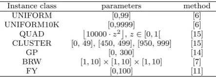
For our experiments we consider seven classes of instances used in the literature.
The first class includes the instances proposed by Balas and Saltzman [6]. The integer cost coefficients ci,j,k are generated uniformly in the interval [0,100]. These instances are denoted as UNIFORM instances.
The instances of the second class are generated using again the method in [6], the only difference being that the cost coefficients are generated uniformly in the interval [0,9999]. We denote these instances as UNIFORM10K.
The third class of instances consists of the 18 instances from Crama and Spieksma [11]. These include are 9 instances size 33 and 9 instances of size 66. In these instances, the cost function is decomposable and the details on the generation procedure can be found in [11]. The fourth and fifth classes of instances are taken from H¨ofler and F¨ugenschuh [15] and denoted as QUAD and CLUSTER respectively. The QUAD instances are randomly gener-ated, with their cost coefficients having a value 10000·z2 wherez is uniformly distributed in the interval [0,1]. The cost coefficients of the CLUSTER instances are chosen out of three clusters [0,49],[450,499],[950,999], where each coefficient lies in a specific cluster with probability equal to 1/3 and is then chosen uniformly from the range of that cluster.
The sixth class of instances, denoted as BRW, is generated using the method described in Burkard et al. [7]. Each cost coefficient is decomposable, assuming the formci,j,k=ai·bj·ck, where each ofai, bj, ck is uniformly distributed in the interval [1,10].
The last class of instances, denoted as GP, is generated using the algorithm proposed in Grundel and Pardalos [14] with random costs coefficients selected uniformly from the interval [1,300]. A detailed explanation on the generation of the cost coefficients can be found in [14].
Instance class parameters method
UNIFORM [0,99] [6]
UNIFORM10K [0,9999] [6]
QUAD
10000·z2
,z∈[0,1[ [15] CLUSTER [0, 49], [450, 499], [950, 999] [15]
GP [0, 300] [14]
BRW [1,10]×[1,10]×[1,10] [7]
[image:15.595.160.382.88.167.2]FY [0,100] [11]
Table 1 Problem classes
7.2 Implementation details
There are different ways of implementing a cutting plane algorithm. For instance, one can add a single violated inequality or all violated ones in each iteration. Although having experimented with both options, we only report the results of the implementation where all violated inequalities are added per iteration. This is because, when adding a single inequality, the inequality found by our separation algorithms may differ from the violated inequality found by the traditional algorithms, thus yielding a different number of iterations and hence a less transparent comparison.
Further, we opt for the following strategy: first, we separate (and add to the LP-relaxation) clique inequalities of type I; next, we separate clique inequalities of type II only if no violated type I inequalities are detected (see Algorithm 7). Of course, this procedure favors the detection of violated type I inequalities.
Algorithm 7Algorithm Outline 0. Let lp = LP relaxation of (2)-(5) 1. Solve lp and findsup(x∗)
2. Inputsup(x∗) to separation algorithm for clique inequalities of type I
ifviolated clique inequalities of type I have been foundthen
update lp by adding all violated clique inequalities of type I; goto step 1
else
Inputsup(x∗) to the separation algorithm for clique inequalities of type II
ifviolated clique inequalities of type II have been foundthen
update lp by adding all violated clique inequalities of type II; goto step 1
end if
STOP: if no violated clique inequalities of type I or type II
end if
Clearly, when implementing Algorithm 7 (see line 1), we need to find the support, i.e., we need to detect which entries are nonzero.To do that we use a tolerance level of 1.0e−05. We ran the experiments with other tolerance levels, and found no significant differences.
7.3 Results and discussion
algorithms by BQ. The first and second columns specify the class and the size of the instances. The third and fourth columns are times taken by DMS and BQ, respectively . The time reported for each size and class is the average time over the 5 (4 for each size of UNIFORM class) instances of that size (and class). The last column gives the average number of cuts added for DMS. Clearly, the LP-bound found by the two separation algorithms is identical; however, the total number of cuts added by both separation algorithms can be different. The reason for this is that, after the first iteration, CPLEX may find different LP solutions (albeit with the same LP value, of course) which is caused by the fact that even if the set of violated inequalities is the same for both separation algorithms, the order in which these inequalities are added to the formulation can be different, and this may influence the LP solution found by the CPLEX. Indeed, when we sorted the inequalities found, and added them in the same order to the formulation, the total number of cuts found by the two separation algorithms is identical. Sorting the inequalities, however, slightly increases the running time, and we chose not to do this. Moreover, we found that the total number of cuts for both implementations differs only marginally; so, we chose to report the average number of cuts for DMS.
Further, since our main focus is on running times of the separation algorithms, we do not report the increase of the LP value (recall that we solve the 3-index assignment as a minimization problem).
Surprisingly, no violated clique inequalities of type II are found in almost all instances. Only in 3 instances, namely 2 from the BRW class and 1 from there UNIFORM class, there have been violated clique inequalities of type II. For this reason, we only report the average number of cuts added. Although this behavior appears uncommon at first sight, similar behavior has been observed for other problems, e.g., for the node packing problem regarding clique and odd-hole inequalities [20]. This may be caused (partly) by the set-up of the separation routine, i.e., there would violated clique of type II if separated before cliques of type I. However, recall that Algorithm 6 relies on the fact no clique inequality of type I is violated in order to exploit the property that any three variables in a clique inequality of type II appear in a clique inequality of type I (and thus improve significantly its running time compared to the traditional algorithm).
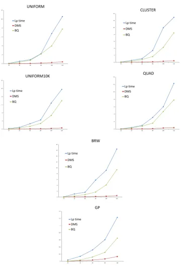
The results of Table 2, show that DMS outperforms BQ in all instances, the improvement being more impressive as the size of the instance grows. Also, compared to BQ the variance in running time is also low for DMS. Thus, also in practice, exploiting sparsity yields separation algorithms that are much faster, often by an order of magnitude: on average, DMS is more than 15 times faster than BQ. This behavior is better illustrated in Figure 3 (whose y-axis reports the average overall classes per size). This shows thatT indeed grows very slowly compared to then3 and in general scales-up pretty well.
8 Conclusion
In this paper we have revisited the idea of exploiting sparsity in separation algorithms. We have also suggested to express the time complexity of such algorithms in terms of sparsity (i.e., the number of non-zero entries in the input). By allowing the input vector of a sepa-ration algorithm to be described by its support, we have obtained more efficient sepasepa-ration algorithms for the clique inequalities of the 3-index assignment problem.
Indeed, the improvement achieved for the 3-index axial assignment problem is significant if the vectors to be separated are vertices of the LP-relaxation because the corresponding formulation contains more variables than constraints. Therefore, analogous improvements could be plausible for other problems whose formulations share this property. However, notice that for problems where column generation is used to solve a linear programming formulation, this idea seems not applicable, since, in such a setting, variables are generated instead of violated inequalities. Thus, formulations with more variables than constraints that are not being solved by a column generation approach are susceptible to the design of efficient separation algorithms that exploit sparsity.
Acknowledgement
We are thankful to Armin F¨ugenschuh for providing the routines to generate instances used in [15], and to Yves Crama for stimulating discussions on this subject.
Type size DMS BQ DMS BQ cuts
Avg Avg Stdev Stdev (#)
CPU(s) CPU(s)
UNIFORM 25 0.006 0.021 0.008 0.008 5.25
54 0.037 0.35 0.023 0.052 8.5
66 0.054 0.764 0.019 0.054 7
80 0.152 2.195 0.023 0.232 8.67
100 0.262 4.008 0.060 0.872 10.4
120 0.408 7.799 0.126 0.804 10.6
QUAD 25 0.004 0.019 0.007 0.018 6.4
54 0.032 0.331 0.009 0.017 7
66 0.065 0.785 0.021 0.031 7.75
80 0.124 1.603 0.052 0.434 14.2
100 0.307 4.74 0.110 0.780 12.8
120 0.382 7.836 0.085 0.608 13.4
BRW 25 0.004 0.022 0.013 0.008 7.6
54 0.043 0.371 0.017 0.028 16.6
66 0.083 0.814 0.041 0.054 17.2
80 0.166 1.729 0.047 0.124 19.4
100 0.265 4.161 0.135 1.454 17.75
120 0.487 9.379 0.118 3.059 21.2
n
0 25 54 66 80 100 120
1 2 3 4
DMS BQ
T ime(s) 10
[image:18.595.143.408.89.252.2]Fig. 3 DMS vs BQ with increasingn
Table 2 – continued from previous page
Type size DMS BQ DMS BQ cuts
UNIFORM10K 25 0.003 0.018 0.011 0.007 6.6
54 0.027 0.307 0.015 0.017 4.6
66 0.051 0.693 0.022 0.027 5.8
80 0.089 1.407 0.026 0.433 4.6
100 0.159 3.368 0.041 0.480 5.6
120 0.293 7.03 0.077 0.696 7
CLUSTER 25 0.004 0.024 0.007 0.018 7.4
54 0.037 0.313 0.013 0.039 9.2
66 0.074 0.788 0.024 0.046 10.2
80 0.148 1.673 0.019 0.152 15.6
100 0.313 4.323 0.077 0.448 13
120 0.446 8.505 0.104 0.655 13.8
GP 25 0.003 0.004 0.007 0.007 6.4
50 0.014 0.038 0.009 0.023 7.5
66 0.035 0.121 0.015 0.046 9.4
80 0.067 0.251 0.028 0.146 13
100 0.1326 0.6488 0.007 0.052 16.2
FY 33 0.006 0.019 0.007 0.008 0.89
66 0.031 0.224 0.009 0.015 2.45
[image:18.595.117.422.311.557.2]References
1. R. Alvarez-Valdes, F. Parreo, and J. Tamarit. A branch-and-cut algorithm for the pallet loading problem.
Computers and Operations Research, 32:3007–3029, 2005.
2. G. Appa, D. Magos, and I. Mourtos. On multi-index assignment polytopes. Linear Algebra and its Applications, 416:224–241, 2006.
3. D. Applegate, R. Bixby, V. Chv´atal, and W. Cook.The Traveling Salesman Problem: A Computational Study. Princeton University Press, ISBN 978-0-691-12993-8, Princeton, New Jersey, 2006.
4. E Balas and L Qi. Linear-time separation algorithms for the three-index assignment polytope. Discrete Applied Mathematics, 43:1–12, 1993.
5. E. Balas and M. Saltzman. Facets of the three-index assignment polytope.Discrete Applied Mathemat-ics, 23:201–229, 1989.
6. E. Balas and M. Saltzman. An algorithm for the three index assignment problem. Operations Research, 39:150–161, 1991.
7. R. Burkard, R. Rudolf, and G. Woeginger. Three-dimensional axial assignment problems with decom-posable cost coefficients. Discrete Applied Mathematics, 65:123–139, 1996.
8. A. Caprara and J. Salazar. Separating lifted odd-hole inequalities to solve the index selection problem.
Discrete Applied Mathematics, 92:111–134, 1999.
9. E. Cheng and W. Cunningham. Separation problems for the stable set polytope. InProceedings of The 4th Integer Programming and Combinatorial Optimization Conference Proceedings, 1995.
10. E. Cheng and W. Cunningham. Wheel inequalities for stable set polytopes.Mathematical Programming, 77:389–421, 1997.
11. Y. Crama and F. Spieksma. Approximation algorithms for three-dimensional assignment problems with triangle inequalities.European Journal of Operational Research, 60:273–279, 1992.
12. J. Van den Akker, C. van Hoesel, and M. Savelsbergh. A polyhedral approach to single machine scheduling problems.Mathematical Programming, 85:541–572, 1999.
13. T. Dokka. Algorithms for multi-index assignment problems. PhD thesis, KU Leuven, 2013.
14. D. Grundel and P. Pardalos. Test problem generator for the multidimensional assignment problem.
Computational Optimization and Applications, 30(2):133–146, 2005.
15. B. H¨ofler and A. F¨ugenschuh. Parametrized grasp heuristics for three-index assignment. EvoCOP, Lecture Notes in Computer science, 3906:61–72, 2006.
16. K. Kaparis and A. Letchford. Separation algorithms for 0-1 knapsack polytopes. Mathematical Pro-gramming, 124:69–91, 2010.
17. J. Kececioglu, Hans-Peter Lenhof, K. Mehlhorn, P. Mutzel, K. Reinert, and M. Vingron. A polyhedral approach to sequence alignment problems.Discrete Applied Mathematics, 104(1-3):143–186, 2000. 18. M. Landete L. Escudero and A. Mar`in. A branch-and-cut algorithm for the winner determination
problem.Decision Support Systems, 46:649–659, 2009.
19. D. Magos and I. Mourtos. Clique facets of the axial and planar assignment polytopes. Discrete Opti-mization, 6:394–413, 2009.
20. G.L. Nemhauser and G. Sigismondi. A strong cutting plane/branch-and-bound algorithm for node packing.Journal of the Operational Research Society, 5:443–457, 1992.
21. L. Qi and D. Sun. Polyhedral methods for solving three index assignment problems.Nonlinear Assign-ment Problems: Algorithms and Applications, P.M. Pardalos and L. Pitsoulis, eds., Kluwer Academic Publishers, Dordrecht, pages 91–107, 2000.
22. S. Rebennack, M. Oswald, D. Oliver Theis, H. Seitz, G. Reinelt, and P. Pardalos. A branch and cut solver for the maximum stable set problem. Journal of Combinatorial Optimization, 21(4):434–457, 2011.
23. A. Schrijver. Combinatorial Optimization, Polyhedra and Efficiency . Springer, 2003.
0 2 4 6 8 10 12
25 54 66 80 100 120
Lp time DMS BQ UNIFORM 0 2 4 6 8 10 12
25 54 66 80 100 120
Lp time DMS BQ UNIFORM10K 0 2 4 6 8 10 12 14
25 54 66 80 100 120
Lp time DMS BQ CLUSTER 0 2 4 6 8 10 12 14
25 54 66 80 100 120
Lp time DMS BQ QUAD 0 2 4 6 8 10 12 14 16 18
25 54 66 80 100 120
Lp time DMS BQ BRW GP 0 0.2 0.4 0.6 0.8 1 1.2 1.4
25 54 66 80 100
Lp time DMS BQ
[image:20.595.76.467.85.624.2]