The Principal Component Transform of Parametrized Functions

http://www.scirp.org/journal/am ISSN Online: 2152-7393

ISSN Print: 2152-7385

The Principal Component Transform of

Parametrized Functions

Ilia Zabrodskii, Arcady Ponosov

Department of Science and Technology, Norwegian University of Life Sciences, Å s, Norway

Abstract

Many advanced mathematical models of biochemical, biophysical and other processes in systems biology can be described by parametrized systems of nonlinear differential equations. Due to complexity of the models, a problem of their simplification has become of great importance. In particular, rather challengeable methods of estimation of parameters in these models may re-quire such simplifications. The paper offers a practical way of constructing approximations of nonlinearly parametrized functions by linearly parame-trized ones. As the idea of such approximations goes back to Principal Com-ponent Analysis, we call the corresponding transformation Principal Compo-nent Transform. We show that this transform possesses the best individual fit property, in the sense that the corresponding approximations preserve most information (in some sense) about the original function. It is also demon-strated how one can estimate the error between the given function and its ap-proximations. In addition, we apply the theory of tensor products of compact operators in Hilbert spaces to justify our method for the case of the products of parametrized functions. Finally, we provide several examples, which are of relevance for systems biology.

Keywords

Principal Component Analysis, Discretization of Functions, Metamodeling, Latent Parameters

1. Introduction

This study is closely related to applications in the so-called “metamodeling” of differential equations, where a “proper” model of an e.g. complex biological process is replaced by its approximation which contains “most information” about the model, but which is simpler. In particular, the true parameters of the model are replaced by “the latent parameters”, which makes the model linear How to cite this paper: Zabrodskii, I. and

Ponosov, A. (2017) The Principal Compo-nent Transform of Parametrized Functions. Applied Mathematics, 8, 453-475.

https://doi.org/10.4236/am.2017.84037 Received: February 23, 2017

Accepted: April 21, 2017 Published: April 24, 2017 Copyright © 2017 by authors and Scientific Research Publishing Inc. This work is licensed under the Creative Commons Attribution International License (CC BY 4.0).

with respect to the latter and hence enables the usage of the (if necessary, partial) least-squares regression. This explains why this idea proved to be efficient in pa-rameter estimation (see e.g. [1]). This also justifies the high numerical efficiency of metamodeling, which has been widely used in statistics [2], chemometrics [3], biochemstry [1], genetics [4] [5] [6], infrared spectroscopy [7] to simplify theo-retical and computational analysis of the “true” models.

Let x=x u

(

,ω

)

be a function, where u∈ ⊂U N and ω∈ Ω, _{Ω ⊂}M being a space of parameters and k∈ be a given number. The kth Principal

Component Transform (PCT) is a specially constructed parametrized function

( )

PCT x k, ≡x_k of the form

( ) ( )

1 k

k i i

i

x p u t ω

=

=

∑

. The image xk is constructed

to yield the minimum distance (in some sense) between x and all possible ap-proximations of x of the form

( ) ( )

1 k

i i

i

z u y ω

=

∑

. The distance is chosen to

en-sure an efficient way to estimate the deviation of xk from x.

Geometrically, the parametrized function x may be regarded as a curve

( )

,

x

ω_ ⋅ω _{in a separable Hilbert space. Then} x_k =PCT

( )

x k, can be inter-

preted as a projection of this curve onto an k-dimensional subspace, which is

chosen in such a way that the image xk gives a best possible individual fit to x

among all k-dimensional subspaces. As we will see in Subsection 3.1, this

nec-essarily leads to nonlinearity of the mapping PCT.

As we will see in Subsection 3.3, discretizing the function x u

(

,ω

)

and its

PCT yields matrices and the projections onto their first k principal compo-

nents, respectively. This explains our terminology: PCT can be regarded as a functional analog of the principal component analysis (PCA) of matrices. This terminology was suggested by Prof. E. Voit in a private talk with the second au-thor during his seminar lecture in Oslo in 2014.

All the papers cited above concentrate on efficiency of the metamodeling ap-proach and disregard mathematical properties of PCT and their justification, which is, for instance, quite important for understanding the limitations of the method and describing the exact conditions under which the method is applica-ble. In particular, the convergence properties of the sequence of metamodels to the original model has not been studied in the available literature. In our paper we try to fill this gap suggesting a rigorous mathematical approach to PCT and analysis of its basic properties. More precisely, we demonstrate how the theory of compact operators in separable Hilbert spaces can be used to provide such an analysis.

products and therefore the product of parametrized functions (Subsection 4.2) and give some examples (Subsection 4.3). In Appendix 5 we offer short proofs of some auxiliary results used in the paper: Allahverdiev’s theorem (Subsection 5.1) and some propositions related to tensor products of linear compact operators in Hilbert spaces (Subsection 5.2).

2. The Best Individual Fit Theorem

In this section we define the distance in the space of parametrized functions and describe how best individual fits PCT

( )(

x k, k∈

)

to a given function x can be obtained using the theory of compact operators in Hilbert spaces. We also prove nonlinearity and continuity of PCT and give some specific examples.

2.1. The Distance in the Space of Parametrized Functions

Let U be a compact subset of N and Ω be a compact subset of M. We

consider the separable Hilbert spaces 2

( )

L U and 2

( )

L Ω with the standard

scalar products

( )

⋅ ⋅, and the norms ⋅ .

Suppose we are given a measurable, square integrable function x: U× Ω →,

i.e.

(

)

2

, d d

U

x uω u ω

Ω

< ∞

∫∫

(1)

The aim is to find a best possible approximation of x in the class k of all

functions of the form

(

)

( ) ( )

1

,

k

k i i

i

x uω z u y ω

=

=

∑

, where 2

( )

i

z ∈L U and

( )

2

i

y ∈L Ω .

To explain better the nature of topology we use in this case let us have a look at finite dimensional Hilbert, i.e. Euclidean, spaces. Let X =   xij be an m n×

-matrix, for instance, a discretized function x u

(

,ω

)

where xij =x u

(

i,

ω

j

)

. In

this case, the best approximation Xk to X in the class of m n× -matrices of

rank not greater than k is given by the first k terms in the singular value

de-composition of X:

*

1

,

k

k i i

i

X t p

=

=

∑

₍₂₎

where ti =Xpi and pi are the normalized eigenvectors of the matrix

*

X X

and *

A is the conjugate (transpose) of a matrix A. In other words,

min X−Y = X−X_k , where rank Y ≤k (3)

The matrix norm is defined as

1

sup

Z Z

α≤ α

= _{, where} α _{is the Euclidean}

norm in n.

Now we will look at arbitrary real separable Hilbert spaces which are denoted by H and K and which are equipped with the scalar products

( )

⋅ ⋅, _H and

( )

,

K

⋅ ⋅ _{and the corresponding norms}

H

⋅ _and

K

⋅ _{, respectively. Assume that}

:

X H →K is a linear compact operator. Its norm is again defined as

1

sup

H

K

X X

α ≤ α

Put

(

,

)

{

is a linear bounded operator from to such that dim Im

(

)

}

k H K = Y H K Y ≤k

 (4)

We want to find an operator X_k∈_k

(

H K,

)

for which X −X_k →min.

The construction of Xk is very close to the singular value decomposition of

matrices.

Assume that *

:

X H→K is the adjoint of X. Then the linear compact

op-erators *

: ,

X X H→H *

:

XX K→K are self-adjoint and positive-definite.

Let 2 2 2

(

)

1 2 i 0, i 0, 1, 2,i

σ

≥

σ

≥≥

σ

≥→

σ

> =  be all positive eigen- values of the operator _{X X}* , the associated normalized eigenvectors being

1, 2, 3,

p p p ∈H, respectively:

* 2

, 1,

i i i i H

X Xp =σ p p = i∈ (5)

It is well-known that pi can always be chosen to be orthogonal:

,

i j

p ⊥ p i≠ j and for any α∈H there is a unique set c_i∈, i∈ and a

unique

(

*

)

0 Null

p ∈ X X for which ₀

1 i i i

p c p

α ∞

=

= +

∑

and, moreover, 2

2 2

0 1

.

i

H H

i

p c

α ∞

=

= +

∑

Now, the operator X can be represented as

(

)

1

, i H i,

i

Xα α p t

∞ =

=

∑

(6)

where ti =Xpi and the convergence is understood in the sense of the norm in

the space K. The truncated versions X_k∈_k

(

H K,

)

of this representation is

defined by

(

)

1

,

k

k i H i

i

X α α p t

=

=

∑

₍₇₎

The following result, a short proof of which is offered in Appenix 5.1, is known as Allahverdiev’s theorem, see e.g. [8, Chapter II, p. 28]:

Theorem 1. For any linear compact operator X H: →K

( ) 1

,

min k k

Y∈_k H K X−Y = X−X =

σ

+ (8)

The functions in numerical calculations are usually replaced by their discreti- zations, which in the case of parametrized functions gives matrices. That is why, the distance in the space of the parametrized functions x u

(

,ω

)

should be

con-sistent with the distance in the space of matrices, so that we can get all the ad-vantages of the finite dimensional singular value decomposition as well as Al-lahverdiev’s theorem. To define the distance in the space of matrices we have to interpret matrices as linear operators between two Euclidean spaces. Analo- gously, we have to interpret parametrized functions as operators between suita-ble Hilbert spaces, and define the distance accordingly.

Let us therefore go back to the spaces 2

( )

L U , L2

( )

Ω , where U, as before,

is a compact subset of N and Ω is a compact subset of

.

M

(

)( )

(

,

) ( )

d

U

Xα ω =

∫

x uω α u u (9)

Under the assumptions of the square integrability of the kernel x u

(

,ω

)

the

operator X becomes compact and linear from the space L U2

( )

to the space

( )

2

L Ω (see e.g. [9], Chapter 7, p. 202]).

The distance between two square integrable parametrized functions x and

x′ can be now defined in the following way:

(

)

dist x x, ′ = X −X′, (10)

where X is defined in (9) and

(

)( )

(

,

) ( )

d .

U

X′α ω =

∫

x u′ ω α u u The norm of

the linear operators acting from 2

( )

L U to L2

( )

Ω is defined in the standard

way.

Remark 1. Evidently,

(

)

2

, d d

U

X C x uω u ω

Ω

≤

_∫∫

₍₁₁₎

for some constant C. Therefore, L2-convergence of the sequence

{ }

x( )n

im-plies the convergence in the sense of the distance dist.

Let * 2

( )

2

( )

:

X L Ω →L U be the adjoint of X, so that

(

*

)

( )

(

) ( )

, d

X β u x uω β ω ω

Ω

=

_∫

(12)

Now, the self-adjoint and positive-definite integral operators

( )

( )

( )

( )

* 2 2 * 2 2

: and :

X X L U →L U XX L Ω →L Ω (13)

can be written as follows:

(

*

)

( )

( ) ( )

( )

(

) (

)

, d , where , , , d

U

X Xα u γ u v α v v γ u v x uω x vω ω

Ω

=

_∫

=

_∫

(14)

and

(

*

)

( )

(

) ( )

(

)

(

) (

)

, d , where , , , d ,

U

XX β ω δ ω ξ β ξ ξ δ ω ξ x uω x uξ u

Ω

=

_∫

=

_∫

(15)

respectively. Let, as before,

(

)

2 2 2

1 2 i 0 i 1, 2,

σ

≥

σ

≥≥

σ

≥→ =  (16)

be all positive eigenvalues of the integral operator (14) associated with its nor-malized and mutually orthogonal eigenfunctions 2

( )

i

p ∈L U , i.e.

( )( )

( ) ( )

2

( )

( ) ( )

0

(

₍

)

₎

, d , d

1

i i i i i j

U U

i j

p u u v p u u p u p u p u u

i j

γ σ  ≠

Γ = = =  ₌



∫

∫

(17)

From Theorem 1 we immediately obtain the Best Individual Fit Theorem. Theorem 2. For a given function x U: × Ω → satisfying (1) the best

ap-proximation of x in the class k of all functions of the form

( ) ( )

1 k

i i

i

z u y ω

=

∑

,

where 2

( )

i

z ∈L U and yi∈L2

( )

Ω , is given by

(

)

( ) ( )

1

, ,

k

k i i

i

x uω p u t ω

=

where pi are the normalized, mutually orthogonal eigenfunctions of the

oper-ator (14) and i

( ) (

i

)( )

(

,

) ( )

i d

U

t ω = Xp ω =

∫

x uω p u u. Moreover,

(

)

1

dist x x, k =σk+ for all natural k.

In other words,

(

)

(

)

1

dist x y, ≥dist x x, _k =σ_k+ for all y∈_k (19)

Remark 2. The functions ti have the following properties (which we do not

use in this paper):

• ti ⊥tj for all i≠ j;

• ti =σi for all i;

• * 2

i i i

XX t =σ t for all i.

Definition 1.

• The kth Principal Component Transform (PCT) of the function 2

(

)

x∈L U× Ω

is defined as

( )(

)

(

)

( ) ( )

1

PCT , , ,

k

k i i

i

x k uω x u ω p u t ω

=

= =

∑

(20)

• The Full Principal Component Transform of the function 2

(

)

x∈L U× Ω is

given by

(

)(

)

( ) ( )

1

PCT , , _{i i}

i

x uω p u t ω

∞ =

∞ =

∑

(21)

We will also write PCT

(

x,∞ ≡

)

PCT

( )

x .

We remark that none of these transforms is uniquely defined: even if all σi

are all different, we have always a choice between two normalized eigenfunctions

i

p . However, the distance between x and any x_k is independent of the

pro-jection we use. On the other hand, this means that the properties of PCT should be formulated with a care.

2.2. Examples of PCT

In this subsection we consider three examples which are of importance in sys-tems biology.

Example 1. Let

(

,

)

x u

ω

=uω (22)

Assume that u∈

[ ]

a b, , ,a b∈,a>0,ω∈

[ ]

0,1 . Then, using Formulas (14)

and (15), we obtain the following representations of the kernels γ _and δ

( )

1 1

( )

_{( )}

0 0

1

, d d ,

ln

uv

u v u v uv

uv

ω ω ω

γ =

_∫

ω=

_∫

ω= − (23)

(

,

)

d d 1 1

1

b b

a a

b a

u u u u u

ω ξ ω ξ

ω ξ ω ξ

δ ω ξ

ω ξ

+ + + +

+ −

= = =

+ +

∫

∫

(24)

Therefore the normalized eigenfunctions p ui

( )

can be obtained from the equation

( )

( )

( )

1

2

0

1

d

ln i i i

uv

p u u p u

uv

σ

 −  ₌

 

 

 

The functions

( )

( )

d

b

i i

a

t ω =

∫

u p uω u can be alternatively found from the

equ-ations

( )

( )

1 1 1

2

0

d

1 i i i

b a

t t

ω ξ ω ξ

ω ω σ ω

ω ξ

+ + + +

 −  ₌

 _{+ +} 

 

∫

(26)

The parametrized power function xω is of crucial importance in the bioche-

mical system theory, where u represents the concentration of a metabolite, while ω stands for the kinetic order. In the case of several metabolites, one gets products of such power functions, which, in turn, are included into the right- hand side of the so-called “synergetic system”, see (e.g. [10], Chapter 2, p. 51) and the references therein. The products of parametrized power functions are considered in Section 4.

Example 2. Consider the function

(

,

)

u

x u

ω

=e−ω (27)

Assume that u∈ −

[

c c,

]

, c∈,c>0, ω∈

[ ]

a b, , ,a b∈, a>0. Then, using

Formulas (14) and (15), we obtain the following representations of the kernels γ and δ

( )

( ) 1

(

( ) ( )

)

, d d ,

b b

u v a u v b u v

u v

a a

u v e e e e e

u v

ω

ω ω

γ ₌ − − ω₌ − + ω₌ − + ₋ − +

+

∫

∫

(28)

(

)

( )

, d d

c c

u l u u l

c c

eω e u e ω u

δ ω ξ − − − +

− −

=

_∫

=

_∫

₍₂₉₎

We denote for simplicity

(

)

( )

( )

( )

0

1

for 0

, , d

1

for 0

s l s

u

s

e s

l

F s e u

e s

l

ω

ω ξ

ω ξ ω

ω ξ

ω

+ − +

− +

 _<

 +

= = 

 _>

 + 

∫

(30)

and get

(

,

)

F c

(

, ,

)

F

(

c, ,

)

δ ω ξ = ω ξ − − ω ξ (31)

Therefore the normalized eigenfunctions p ui

( )

can be obtained from the equation

( ) ( )

(

)

( )

2

( )

1

d

a

a u v b u v

i i i

b

e e p u u p u

u v

σ

− + − +

 

− =

 

 ₊ 

 

∫

(32)

The functions

( )

( )

d

b u

i i

a

t ω =

∫

e−ω p u u can be also obtained from the

equa-tions

(

)

(

)

(

)

( )

2

( )

, , , , d

c

i i i

c

F cω ξ F cω ξ t ω ω σ t ω

−

− − =

∫

(33)

The function u

e−ω is often used in the neural field models, where it serves as

Example 3. Consider the Hill function

(

,

)

q

q q

u x u

u

ω

θ

=

+ (34)

Assume that u∈

[ ]

a b, , ,a b∈, > 0a , q∈

[

q q₀, _m

]

, q q₀, _m∈, q₀>0,

[

0, m

]

, 0, m , 0 0.

θ∈θ θ θ θ ∈ θ > Putting ω=

(

q,θ

)

and ξ=

(

q′ ′,θ

)

we

ob-tain

( )

0 0

, d d

m m

q q q

q q q q q

u v

u v q

u v

θ

θ

γ θ

θ θ

=

+ +

∫ ∫

(35)

and

(

,

)

d

b q q

q q q q a

u u

u

u u

δ ω ξ

θ θ

′

′ ′

=

′

+ +

∫

(36)

The Hill function plays central role in the theory of gene regulatory networks, where it stands for the gene activation function, x being the gene concentra- tion and θ _{being the activation threshold, see e.g. [12] and the references} therein.

3. Some Properties of PCT

The Principal Component Transform PCT

( )

x k, is not uniquely defined. That

is why, we will use a special notation when comparing PCT of different func- tions, namely, we will write PCT

( )

x k, = PCT

(

y k,

)

if there exist coinciding

versions of PCT of x and y.

3.1. PCT Is Homogeneous, But Not Additive

Theorem 3.

1. PCT

(

cx k,

)

=cPCT

( )

x k, for any c∈ and k∈.

2. In general,

(

( )1 ( )2

)

PCT x +x ,k is different from PCT

(

x( )1,k

)

+PCT

(

x( )2 ,k

)

.

Proof.

1. The case c=0 is trivial. We assume therefore that c≠0. Let

(

)( )

(

,

) ( )

d

U

Xα ω =

∫

x uω α u u and

( )(

)

( ) ( )

1

PCT , i i

i

x uω p u t ω

∞ =

=

∑

, see (21). By

definition, pi are normalized, mutually orthogonal eigenfunctions of the ope-

rator *

X X and ti =Xpi. Let Xc

( )

α ≡ X c

( )

α . Then

( ) ( )

* * 2 * 2 2

,

c c i i i i i i

X X p =X cp X cp =c X Xp =c

σ

p (37)

so that pi are the same for Xc and X. On the other hand,

( )

( )

( )

c i i i i

X p = X cp =cX p =ct and

(

)(

)

( ) ( )

( )(

)

1

PCT , , PCT , ,

k

i i

i

cx k u ω p u ct ω c x k u ω

=

=

∑

=_{ (38)}

2. Before constructing an example illustrating nonlinearity of PCT we remark that this statement, in its more precise formulation, says that there are no versions of

(

( )1 ( )2

)

( ) ( )

(

1 2

)

(

( )1

)

(

( )2

)

PCT x +x ,k =PCT x ,k +PCT x ,k .

Let U = Ω =

[ ]

0,1 and the functions rτ: 0,1

[ ]

→

(

τ=1, 2

)

satisfy

( )

( ) ( )

1 1

2

1 2

0 0

d 1 and d 0

r_τ u u= r u r u u=

∫

∫

(39)

We put ( )

(

)

( )

( ) ( ) ( )

( ) ( ) ( )

( )

(

)

( )

(

( )

( )

)

( )

( )

(

( )

( )

)

( )

1 1

1

1 1 2 2

0 0

1 1

2

1 1 2 2 1 2

0 0

2 d ,

( ) 2 d d .

X r r u u du r r u u u

X r r u r u u u r r u r u u u

α ω ω α ω α

α ω ω α ω α

= +

= + + +

∫

∫

∫

∫

(40)

To calculate PCT we observe that both operators have a 2-dimensional image in 2

( )

L Ω . Using the representation α

( )

u =c r u1 1

( )

+c r u2 2

( )

+αˆ

( )

u where

(

)

ˆ rτ 1, 2

α⊥ τ= we reduce the operators ( )1

X and X( )2 to the matrices

2 0 2 1

and , respectively,

0 1 1 2

A=_ _ B=_ _

   

so that

( )1

_{( ) (}

₎

* ( )2

_{( ) (}

₎

*

1 2 1 2 and 1 2 1 2 ,

X

α

= r r A c c X

α

= r r B c c (41)

where

( )

a b, and

( )

a b, * are row and column vectors, respectively.

Matrices A and B are symmetric. Then * 2

A A=A and B B* =B2. The

first eigenpairs of 2

A and B2 are 4, 10

( )

* and 9, 11

( )

*, respectively. There-

fore the best rank 1 approximations of A and B are

1 1

2 0 1.5 1.5

and , respectively,

0 0 1.5 1.5

A =_ _ B =_ _

   

so that

(

( )1

)

(

)

( ) ( )

1 1

PCT X ,1 u,ω =2r u r ω and

( )

(

2

)

(

)

(

( )

( )

)

(

( )

( )

)

1 2 1 2

PCT X ,1 u,ω =1.5 r u +r u r ω +r ω , which both are

operators with an 1-dimensional image. However, their sum

( ) ( )

( ) ( )

( ) ( )

( ) ( )

1 1 1 2 2 1 2 2

3.5r u r ω +1.5r u r ω +1.5r u r ω +1.5r u r ω (42)

has a 2-dimensional image, as its representation in the basis

{

r r1, 2

}

is given by

the non-singular matrix 3.5 1.5

1.5 1.5 A=  _

 . Therefore ( )

(

1

)

(

( )2

)

PCT X ,1 +PCT X ,1 cannot coincide with any version of PCT

(

X,1

)

.

3.2. PCT Is Continuous

Let us consider a sequence of parametrized, square integrable functions ( )n _:

x U× Ω →.

Theorem 4. Let k∈ and dist

(

x( )n,x

)

→0

(

n→ ∞

)

for some parame-

trized, square integrable functions x( )n, :x U× Ω →. Then for any version

( )

,

k

( )

(

)

dist xkn ,xk →0, n→ ∞ (43)

Proof. Let 2

( )

H =L U , K=L2

( )

Ω . We define the compact linear integral

operators X( )n ,X H: →K using the kernels x( )n , respectively. By the

defini-tion of the dist we immediately get that X( )n −X →0, n→ ∞.

Let pi, 1,i= ,k be the normalized, mutually orthogonal eigenfunctions of

the operator *

X X corresponding to its first k eigenvalues 2 2 2

1 2 k

σ ≥σ ≥_≥σ . Since ( )n

X converges to the operator X in norm, we can always choose a

se-quence of the eigenfunctions ( )n i

p such that

( )

0, , 1, ,

n i i

H

p −p → n→ ∞ =i  k (44)

In this case

( ) ( ) ( )

, , 1, ,

n n n

i i i i

t =X p → =t Xp n→ ∞ =i  k (45)

Therefore Xk( )n −Xk →0, n→ ∞, which implies

( )

(

)

dist xkn,xk →0, n→ ∞ (46)

The above theorem can be reformulated in terms of robustness of PCT. Corollary 1. Let k∈ and x U: × Ω → be a parametrized, square inte-

grable function and k∈. Then given an ε>0 there is a ε>0 such that

for every parametrized, square integrable function x′: U× Ω → the follow-

ing holds true:

(

)

(

(

)

( )

)

dist x x′, <

δ

⇒ dist PCT x k′, −PCT x k, <

ε

(47)

for some suitable versions of PCT.

3.3. Discretization of Functions

In the papers [5] [6], which are aimed at applying the metamodeling approach to gene regulatory networks, the approximations of the parametrized sigmoidal functions are performed numerically by using discretization and SVD of the re-sulting matrices. The continuity of PCT, proved in the previous subsection, can now be used to justify this analysis and, in particular, the results on the number of the principal components k ensuring the prescribed precision.

In this subsection we suppose that all functions are continuous, which is suffi-cient for most applications. The general case is, however, unproblematic as well if we slightly adjust the approximation procedure.

Let x be a continuous function on a compact set _D⊂N M+ ,_{D= × ΩU} ,

where s=

(

u,ω

)

.

For all n∈, D is divided into n measurable subsets D_i( )n :

1 n

i i

D D

=

=

_

(48)

We define the sequence of the functions xn

( )

s as follows:

( )

_{( )}

( )

( ) ( )

, ,

n n n

i i

where ( )n i

s is an arbitrary point in Di( )n.

Lemma 1. Let x be a continuous function on D. Then

( )

(

)

dist xn ,x →0, n→ ∞ (50)

provided that ( )

1

max diam in 0

i n D

≤ ≤ → as n→ ∞.

Proof. The function x is continuous on the compact set D, therefore x s

( )

is uniformly continuous on D. Then for all ε >0 there is δ >0 such that

( ) ( )

s−s′ <

δ

⇒ x s −x s′ <

ε

(51)

On the other hand, there is a number N for which ( )

1

max diam in

i n D

ε

≤ ≤ < as

long as n>N . Let s be an arbitrary point from D. Then for any n there is ( )n

i

D such that s∈Di( )n . Taking now an arbitrary n>N we obtain

( )n

_{( ) ( )}

( )

( )n

_{( )}

_, i

x s −x s = x s −x s <ε (52)

so that dist

(

x( )n,x

)

≤Cε, where C2 is the Lebesgue measure of the set D.

Hence dist

(

x( )n ,x

)

→0, n→ ∞.

Corollary 2. Let k∈ and x U: × Ω → be a parametrized, continuous

function,

{ }

( )n

x be a sequence of discrete approximations satisfied the assump-

tions of Lemma 1. Then for any version x_k =PCT

( )

x k, there are versions

( )

(

( )

)

PCT ,

n n

k

x = x k such that dist

(

x( )kn,xk

)

→0, n→ ∞.

Finally, we observe that if ( )n i

D are defined as U( )jn × Ω( )ln , where for any n

( )

{ }

n

j

U and

{ }

Ω( )ln are measurable partitions of U and Ω, respectively, and

( )

,

i= j l , then PCT of the discrete functions x( )n coincide with the k-

trun-cated SVD of the matrix ( )

( )

( ), n

j l

x s

 

 . In the next subsection we provide an

example of such approximation stemming from the biochemical systems theory.

3.4. Examples of Discrete Approximations

In this subsection we study the parametrized power function x u

(

,

ω

)

=uω

de-fined on the interval

[

u u1, n

]

,u u1, n∈,u1>0 with the parameter values

[

1, m

]

.

ω∈ ω ω To approximate this function we construct a matrix X as

fol-lows: we divide

[

u u1, n

]

into n−1 parts: u1<u2<<un. Similarly, we

di-vide the interval

[

ω ω0, m

]

into m−1 parts. Every entry of the matrix X will be given by the values j 1

(

, 1

)

i

uω ≤ ≤i n ≤ ≤j m :

1 1 1

2 2 2

1 2

1 2

1 2

... ...

... ... ... ...

...

m m m

n

n

n

u u u

u u u

X

u u u

ω ω ω

ω ω ω

ω ω ω

 

 

 

=  

 

 

 

 ₍₅₃₎

The corresponding discretization of PCT

( )

x k, will be then given by the

matrix

*

1

, ,

k

n

i i i i

i

t p t p

=

∈ ∈

sition of the matrix X

*

,

m m m n n n

X =U _× S _× P_× (55)

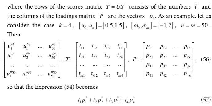
where the rows of the scores matrix T =US consists of the numbers t_i and

the columns of the loadings matrix P are the vectors pi. As an example, let us

consider the case k=4,

[

u u₀, _n

]

=

[

0.5,1.5

]

,

[

ω ω₀, _m

]

= −

[

1, 2

]

, n=m=50.

Then

1 1 1

2 2 2

50 50 50

11 12 13 14 11 12 1

1 1 50

21 22 23 24 21 22 2

1 2 50

31 32 3

1 2 3 4 41 42 4

1 2 50

... ...

... ...

, ,

... ... ... ... ...

... ... ... ...

... ...

n

n

n

m m m m n

t t t t p p p

u u u

t t t t p p p

u u u

X T P

p p p

t t t t p p p

u u u

ω ω ω

ω ω ω

ω ω ω

    

    

    

=_{ } = =

  

    

    

 

 ,

     

(56)

so that the Expression (54) becomes

* * * *

1 1 2 2 3 3 4 4

t p +t p +t p +t p (57)

Assume now that ω=0.5. This value corresponds to row s in the matrix

T. We find a number s as follows:

( )

( )

0

0

0.5 1

50 25

0.5 1

m

s m ω ω

ω ω

− − −

≈ = =

− − − (58)

This yields

1 s1 7.0579 2 s2 0.0089 3 s3 0.2400 4 s4 0.0016

t =t = − t =t = − t =t = t =t =

and hence

( )

( )

( )

( )

0.5 * * * *

1 2 3 4

7.0579 0.0089 0.2400 0.0016

u ≈ − p u − p u + p u + p u (59)

where *

( )

50

, 1, 2, 3, 4

i

[image:12.595.195.540.108.280.2]

p x ∈ i= are the columns in the loadings matrix P, see

Figure 1.

The Figure 1 depicts the power function uω vs. its PCT with 4 components;

[

0.5,1.5 ,

]

[

1, 2

]

u∈ ω∈ − ; the error is estimated as 5

1

0.0001

σ

σ = and the Hill

function 1 1_2.21 q

q q

u

u + vs. its PCT with 12 components;

[

1, 3.5 ,

]

[

0.05,10 ,

]

[

0.01, 5

]

u∈ q∈ θ∈ ; the error is estimated as 13

1

0.0013

σ

σ = .

The Figure 2 depicts the cumulative normal distribution function

1 1 erf

2 2

u µ

θ

 ₊  − 

 _ _

  vs. its PCT with 27 components and

[

2, 2 ,

]

[

0.01, 0.99 ,

]

[

0.1, 0.7

]

u∈ − µ∈ θ∈ ; the error is estimated as 28

1

0.0019

σ

σ =

and the normal distribution function

( )

( )2

2 2 2

1 e

2 π

u

x u

µ θ

θ

− −

= vs. its PCT with

25 PCs; u∈ −

[

2.5,1.5 ,

]

µ∈ −

[

1.5, 0.5 ,

]

θ∈

[

0.1,1

]

; the error is estimated as

26

1

0.0029

σ

[image:13.595.64.538.68.267.2]

(a) (b) Figure 1. (a) The power function and its PCT; (b) The Hill function and its PCT.

(a) (b)

Figure 2. (a) The cumulative normal distribution function and its PCT; (b) The normal distribution function and its PCT.

4. PCT of Products of Functions

To calculate PCT of products of parametrized functions we need to apply the theory of tensor products of Hilbert spaces and compacts operators. Appendix 5.2 includes all the necessary details we need in this section.

Below we use the following notation (where τ=1, 2):

• N

Uτ ⊂ , Ω ⊂τ M are compact sets; • U=U1×U2, Ω = Ω × Ω1 2;

• 2

( )

H_τ =L U_τ , 2

( )

K_τ =L Ω_τ , 2

( )

H =L U , 2

( )

K=L Ω ;

• x( )τ

(

uτ,

ω

τ

)

, uτ∈Uτ , ω ∈ Ωτ τ are square integrable functions and

(

,

)

(

1, 1

) (

2, 2

)

;

x uω =x u ω x u ω

•

(

( )

)

( )

( )

(

,

) ( )

d

U

X h x u h u u

τ

τ τ

τ

ω

τ =

∫

τ

ω

τ τ τ τ so that X( )τ : Hτ →Kτ;

•

( )( )

(

,

) ( )

d

U

[image:13.595.63.538.136.479.2]

4.1. Products of Parametrized Functions

Theorem 5. In the above notation:

• H=H1⊗H2, K =K1⊗K2

• ( )1 ( )2

X =X ⊗X

Proof. We use the definition of the tensor product from Appendix 5.2.

Let 2

( )

H_τ =L U_τ have an orthonormal basis

{

e₁( ) ( ),e₂ , ,ei( ),

}

,

τ τ τ

  so that

any h_τ ∈H_τ can be represented as

( ) ( )

₍

₎

1

1, 2 ,

i i i

hτ c eτ τ τ

∞ =

=

∑

= (60)

where ( )2 1

.

i i

cτ

∞ =

< ∞

∑

We prove now that the set

{

( ) ( )1 2

}

, ,

i j

E≡ e e i j∈ is an orthonormal basis in

the space 2

( )

H =L U . Its orthonormality follows directly from its definition. It

remains therefore to check that the set of all linear combinations of the elements from E is dense in H. Indeed, the set of continuous functions, and hence the

set P of polynomials P u

( )

, on U is dense in H. On the other hand, the

set _Pˆ _{of polynomials of the form} ( )1

( )

( )1 ( )2

( )

( )2

P u P u spans the set P and,

finally, the set E spans the set Pˆ. Thus, E spans H and we have proved

that any h∈H can be represented as the L2-convergent series

( ) ( )1 2

, 1

ij i j i j

h c e e

∞

=

=

∑

₍₆₁₎

for some set cij satisfying

2

, 1

ij i j

c

∞

= < ∞

∑

(62)

Defining

( ) ( )

(

1 2

)

( )

( )1

_{( )}

( )2

_{( )}

1 2

i j i j

e ⊗e u ≡e u e u (63)

and comparing the Representation (61) with the Formula (94) proves the equal-ity H=H1⊗H2. The equality K=K1⊗K2 can be checked similarly.

Let us now prove the last formula of the theorem. First of all, we remark that the Definition (63) implies

( ) ( ) (

)( )

1 1 2 2 1 2

g ω g ω = g ⊗g ω (64)

for any g_τ∈H_τ, 1, 2τ= .

By the assumptions on the kernels, the operators in this equality are linear and bounded. Therefore, it is sufficient to check the equality for h= ⊗h1 h2 (see Appendix 5.2).

( )( )

(

) ( )

( )

₍

₎

( )

₍

_{) ( ) ( )}

( )

₍

_{) ( )}

( )

₍

_{) ( )}

( )

(

)

( )

(

( )

)

_{( )}

(

(

( )

)

(

( )

)

)

_{( )}

1 2

1 1 2 2 1 1 2 2 1 2 1 2

1 2

1 1 1 1 1 2 2 2 2 2

1 2

1 2 1 2

1 1 2 2 1 2

, d

, , d d

, d , d

U U U

U U

Xh x u h u u

x u x u h u h u u u

x u h u u x u h u u

X h X h X h X h

ω ω

ω ω

ω ω

ω ω ω

× =

=

=

= = ⊗

∫

∫

due to (64). Hence

(

)

(

( )1

)

(

( )2

)

1 2 1 2

Xh= X h⊗h = X h ⊗ X h . Comparing this for-

mula with the Definition (100) completes the proof of the theorem.

4.2. PCT Preserves Tensor Products

The main theoretical result of this subsection is the following theorem: Theorem 6.

( ) ( )

(

1 2

)

( )

( )1

( )

( )2

PCT X ⊗X = PCT X ⊗PCT X (66)

Proof. For τ=1, 2 we have by definition

( )

( )

(

( )

)

( )

1

PCT , _{i i} ,

i

X τ α α pτ tτ

∞ =

=

∑

₍₆₇₎

where pi( )

τ

are normalized, mutually orthogonal eigenvectors of the operator ( )

( )

* ( )

Xτ X τ corresponding to the eigenvalues

( )

σ( )τ 2 and t_i( )τ =

( )

X( )τ p_i( )τ .

Put ( )1 ( )2

X =X ⊗X and p_ij = p_i( )1 ⊗p( )_j2 . Using the properties of the tensor

product listed in Appendix 5.2 we obtain

(

)

(

( ) ( )

)

(

( ) ( )

)

(

( ) ( )

)

( )

( )

( )

(

( )

( )

)

(

( ) ( )

)

( )

( )

( ) ( )

( )

( ) ( ) ( ) ( )

( )

( )

( )

( ) ( )

(

( ) ( )

)

1 2 1 2 1 2

* *

1 1 (2) 2 1 2

* *

1 1 1 2 2 2

2 2

1 1 1

*

2 *

2 2

,

ij i j

i j

i i

i i j i i j ij

X X p X X X X p p

X X X X p p

X X p X X p

p p p

σ σ σ σ

= ⊗ ⊗ ⊗

 

=_{ }⊗ ⊗

 

     

=_{   }⊗ _{  }

   

   

   

=  ⊗ =

   

(68)

where

(

)

(

(

( )1 ( )2

)

(

( )1 ( )2

)

)

(

( )1 ( )1

)

(

( )2 ( )2

)

, , , ,

1 if , and 0 otherwise

ij lm i j l m i l j m

p p p p p p p p p p

i l j m

= ⊗ ⊗ =

= = = = (69)

This proves that pij are normalized, mutually orthogonal eigenvectors of the

operator _{X X}* corresponding to the eigenvalues ( ) ( )1 2

i j

σ σ

.

On the other hand,

( ) ( )

(

)

(

( ) ( )

)

( ) ( )

(

)

(

( ) ( )

)

( ) ( )

1 2 1 2

1 1 2 2 1 2

ij i j

i i i j ij

Xp X X p p

X p X p t t t

= ⊗ ⊗

⊗ = ⊗ ≡ (70)

Therefore,

( ) ( )

(

)

(

)

(

)

(

)

( )

(

)

( )

(

( )

)

( )

( )

( )

( )

( )

1 2

1 2 1 2

1 1

1 1 2 2

1 1

1 1

1 2

PCT ,

, ,

PCT PCT ,

ij ij

i j

i i i i

i j

X X p t

p t p t

X X

α α α α

α α

∞ ∞

= =

∞ ∞

= =

⊗ ⊗ = ⊗

 

 

=_{ ⊗  }

   

= ⊗

∑∑

∑

∑





(71)

Remark 3.Theorem 6 is only valid for the full PCT. The truncated versions of PCT are not necessarily valid, as the order of the singular values ( ) ( )1 2

ij i j

σ

=

σ σ

depends on the magnitude of the eigenvales ( )1

i

σ

and ( )2

j

σ

_.

4.3. Examples of Products of Parametrized Functions

In this subsection we describe the kernels of the integral operators related to products of parametrized functions from Subsection 0. These examples are of importance in systems biology.

Example 1. Consider the following function

(

)

1 2

1, 2, 1, 2 1 2 , 1, 2 , 1, 2

x u u

ω ω

=u uω ω u u ∈U

ω ω

∈ Ω (72)

Assume that U=

[ ]

a b, , ,a b∈, a>0, Ω =

[ ]

0,1 . Then, using Formulas (14)

and (15), we obtain the following representations of the kernels γ and δ

(

)

(

) (

)

(

)

(

)

(

) (

)

1 2 1 2

1 2

2 1

1 2 1 2 1 2 1 2 1 2

1 1

1 1 2 2 1 2 0 0

1 1

2 2 2 1 1 1

0 0

1 1 2 2

1 1 2 2

, , , d d

d d

d d

1 1

,

ln ln

u u v v u u v v

u v u v

u v u v

u v u v

u v u v

ω ω ω ω

ω ω

ω ω

γ ω ω

ω ω ω ω Ω = = = − − = ⋅

∫∫

∫∫

∫

∫

(

)

1 2 1 2

1 1 2 2

1 1 2 2

1 1 1 1 1 1 2 2

1 2 1 2 1 2 1 2 1 2

1 2 1 2

1 1 2 2

1 1 1 1

1 1 2 2

, , , d d

d d d d 1 1 U U b b a a c

u u u u u u

u u u u

u u u u

b a b a

ω ω ξ ξ

ω ξ ω ξ

ω ξ ω ξ

ω ξ ω ξ ω ξ ω ξ

δ ω ω ξ ξ

ω ξ ω ξ

+ + + + + + + + + + + + = = = − − = ⋅ + + + +

∫∫

∫∫

∫

∫

Example 2. Consider the function

(

)

1 1 2 2

1, 2, 1, 2 , ,1 2 , ,1 2

u u

x u u

ω ω

=e−ω ⋅e−ω u u ∈U

ω ω

∈ Ω (73)

Assume that U= −

[

c c,

]

, c∈, c>0, Ω =

[ ]

a b, , ,a b∈, a>0. Then,

us-ing Formulas (14) and (15), we obtain the followus-ing representations of the ker-nels γ _and δ

(

)

( ) ( )

( ) ( )

( ) ( )

(

)

1 1 2 2 1 1 2 2

1 1 1 2 2 2

1 1 1 2 2 2

1 2 1 2 1 2

|

1 2

1 2

, , , d d

d d

d d

1

,

u u v v

u v u v

b b

u v u v

a a

b u v a u v

u u v v e e e e

e e

e e

e e

u v

ω ω ω ω

ω ω

ω ω

γ ω ω

(

)

( ) ( )

( ) ( )

(

)(

)

(

( ) ( )

)

(

( ) ( )

)

1 1 2 2 1 1 2 2

1 1 1 2 2 2

1 1 1 2 2 2

1 1 1 1 1 1 2 2 2 2 2 2

1 2 1 2 1 2

1 2

1 2

1 1 2 2

, , , d d

d d

d d

1

u u u u

U

u u

U

c c

u u

c c

u u u u

e e e e u u

e e u u

e u e u

e e e e

ω ω ξ ξ

ω ξ ω ξ

ω ξ ω ξ

ω ξ ω ξ ω ξ ω ξ

δ ω ω ξ ξ

ω ξ ω ξ

− − − − − + − +

− + − +

− −

− + + − + +

=

=

=

= − ⋅ −

+ +

∫∫

∫∫

∫

∫

Example 3. For the Hill function we obtain

(

)

1 2

1 1 2 2

1 2

1 2 1 2

1 1 2 2

, , ,

q q

q q q q

u u

x u u

u u

ω ω

θ θ

=

+ + (74)

Assume that

[ ]

, , , , , 0,

i

u ∈U U = a b a b∈ a>

(

,

)

,

[

0,

]

, 0, , 0,0

i qi i qi q qm q qm q

ω = θ ∈ ∈_ >

[

0,

]

, 0, , 0, 1, 2.0

i m m i

θ ∈θ θ θ θ ∈ θ > =

Putting Ω =

[

q q0, m

] [

× θ θ0, m

]

and ξi =

(

qi′ ′,θi

)

,i=1, 2. Then, using Formu- las (14) and (15), we obtain the following representations of the kernels γ and

δ

(

)

1 2 1 2

1 1 2 2 1 1 2 2

1 2 1 2

1 2 1 2 1 2

1 1 2 2 1 1 2 2

, , , d d ,

q q q q

q q q q q q q q

u u v v

u u v v

u u v v

γ ω ω

θ θ θ θ

ΩΩ =

+ + + +

∫∫

(75)

(

)

1 2 1 2

1 1 2 2 1 1 2 2

1 2 1 2

1 2 1 2 1 2

1 1 2 2 1 1 2 2

, , , d d

q q q q

q q q q q q q q

U

u u u u

u u

u u u u

δ ω ω ξ ξ

θ θ θ θ

′ ′

′ ′ ′ ′

=

′ ′

+ + + +

∫∫

(76)

Remark 4. The eigenfunctions of the integral operators with the kernels that are products of parametrized functions are, according to Subsection 5.2, also products of the respective eigenfunctions of the factors.

5. Conclusions

The main results of the paper can be summarized as follows. We defined the distance in the space of parameterized functions. We defined the k-th Principal

Component Transform (PCT) and the Full Principal Component Transform of

functions 2

(

)

x∈L U× Ω . The kth PCT is the best approximation of the given

function, i.e. it minimizes dist ,

( )

⋅ ⋅ . We proved that if the sequence of functions

( )n

_{( )}

x s converge to the continuous function x s

( )

, then the sequence of the

PCT of ( )n

( )

x s will converge to the PCT of x s

( )

. Some properties of PCT

were considered. These results can also serve as theoretical background for the design of some metamodels. Using the theory of the tensor product of Hilbert spaces and compact operators we calculated the PCT of products of functions. We provided several examples of the discrete approximations and products of the parametrized functions.

We will emphasize that our study is related to systems biology. In future works we aim to investigate the problem of “sloppiness” in nonlinear models [1]

Chapter 2, p. 51).

Acknowledgements

The work of the second author has been partially supported by the Norwegian Research Council, grant 239070.

References

[1] Tafintseva, V., Tøndel, K., Ponosov, A. and Martens, H. (2014) Global Structure of Sloppiness in a Nonlinear Model. Journal of Chemometrics, 28, 645-655.

https://doi.org/10.1002/cem.2651

[2] Tøndel, K., Gjuvsland, A., Måge, I. and Martens, H. (2010) Screening Design for Computer Experiments: Metamodelling of a Deterministic Mathematical Model of the Mammalian Circadian Clock. Journal of Chemometrics, 24, 738-747.

https://doi.org/10.1002/cem.1363

[3] Martens, H., Måge, I., Tøndel, K., Isaeva, J., Gjuvsland, A., Høy, M. and Sæbø, S. (2010) Multi-Level Binary Replacement (MBR) Design for Computer Experiments in High-Dimensional Nonlinear Systems. Journal of Chemometrics, 24, 748-756.

https://doi.org/10.1002/cem.1366

[4] Martens, H., Veflingstad, S.R., Plahte, E., Martens, M., Bertrand, D. and Omholt, S.W. (2009) The Genotype-Phenotype Relationship in Multicellular Pattern-Gene- rating Models—The Neglected Role of Pattern Descriptors. BMC Systems Biology, 3, 87. http://bmcsystbiol.biomedcentral.com/articles/10.1186/1752-0509-3-87 [5] Isaeva, J., Sæbø, S., Wyller, J.A., Liland, K.H., Faergestad, E.M., Bro, R. and Martens,

H. (2010) Using GEMANOVA to Explore the Pattern Generating Properties of the Delta-Notch Model. Journal of Chemometrics, 24, 626-634.

https://doi.org/10.1002/cem.1348

[6] Isaeva, J., Sæbø, S., Wyller, J.A., Wolkenhauer, O. and Martens, H. (2012) Nonli-near Modelling of Curvature by Bi-LiNonli-near Metamodeling. Chemometrics and Intel-ligent Laboratory Systems, 117, 2-12.

[7] Konevskikh, T., Blümel, R., Lukacs, R., Ponosov, A. and Kohler, A. (2015) Fringes in FTIR Spectroscopy Revisited: Understanding and Modelling Fringes in Infrared Spectroscopy of Thin Films. Analyst, 140, 3969-3980.

https://doi.org/10.1039/C4AN02343A

[8] Gohberg, I.C. and Krein, M.G. (1969) Introducion to the Theory of Linear Nonsel-fadjoint Operators in Hilbert Space. American Mathematical Society, Providence. [9] Hutson, V., Pym, J.S. and Cloud, M.J. (2005) Applications of Functional Analysis

and Operator Theory. Elsevier Science, Amsterdam.

[10] Voit, E.O. (2000) Computational Analysis of Biochemical Systems. A Practical Guide for Biochemists and Molecular Biologists. Cambridge University Press, Cambridge.

[11] Burlakov, E., Ponosov, A., Wyller, J. and Zhukovskii, E. (2015) Existence, Unique-ness and Continuous Dependence on Parameters of Solutions to Neural Field Equa-tions. Memoirs on Differential Equations and Mathematical Physics, 65, 35-55. [12] Mestl, T., Plahte, E. and Omholt, S.W. (1995) A Mathematical Framework for

Appendix

1. Allahverdiev’s theorem

Let K and K be two real separable Hilbert spaces, equipped with the

sca-lar products

( )

⋅ ⋅, _H and

( )

⋅ ⋅, _K and the corresponding norms ⋅_H and ⋅_K,

respectively. Assume that X H: →K is a linear compact operator. Its norm is

defined as

1

sup

H

K

X X

α ≤ α

= .

Put

(

,

)

{

is a linear bounded operator from to such that dim Im

(

)

}

.

k H K = Y H K Y ≤k



We want to find an operator X_k∈_k

(

H K,

)

for which X−X_k →min.

This construction is very close to the finite dimensional singular value decom-position.

Assume that *

:

X H→K is the adjoint of X. Then the linear compact

op-erators *

: ,

X X H→H *

:

XX K→K are self-adjoint and positive-definite.

Let 2 2 2

1 2 3 0

σ ≥σ ≥σ ≥_→ _, σ >i 0 be all positive eigenvalues of the operator

*

X X, the associated normalized eigenvectors being p p₁, ₂,p₃,∈H,

respec-tively:

* 2

, 1, .

i i i i

X Xp =

σ

p p = i∈ (77)

It is well-known that pi can always be chosen to be orthogonal:

, .

i j

p ⊥ p i≠ j By the Hilbert-Schmidt theorem, for any α∈H there is a

unique set ci∈ , i∈ and a unique

(

)

* 0 Null

p ∈ X X for which

0 1

i i i

p c p

α ∞

=

= +

∑

and, moreover, 2 2 2

0 1

.

i

H H

i

p c

α ∞

=

= +

∑

Thus, the operator X

can be represented as

(

)

1 1

, _{i i i i},

H

i i

Xα α p t c t

∞ ∞

= =

=

∑

=

∑

₍₇₈₎

where ti =Xpi, and the convergence is understood in the sense of the norm in

the space K. We define the linear bounded operators X_k∈_k

(

H K,

)

by

(

)

1 1

,

k k

k i H i i i

i i

X α α p t c t

= =

=

∑

=

∑

(79)

The following result is known as Allahverdiev’s theorem, see e.g. [8]: Proposition 7. For any linear compact operator X H: →K

( ) 1

,

min

k

k k

Y∈ H K X−Y = X−X =

σ

+ (80)

Proof. First of all, we prove that X−Xk =σk+1. By definition,

(

)

1

2 2

sup

H

k k _K

X X X X

α _≤ α

− = − (81)

From (79) and (78) we get

(

)

1 1 1

k

k k i i i i i i

i i i k

X X α Xα X α c t c t c t

∞ ∞ = = = +

− = − =

∑

−

∑

=

∑

(82)