Abstract—According to many reports from papers and applications, using gradient-based search methods to generate optimum topology in a design space might result in topologies with gray elements and checkerboard structures in some areas. These drawbacks sometimes may cause difficulty to identify genuine optimum topology in the given design space. In order to solve this problem, this research develops some new functions of Young’s modulus related to design variables. These functions are different from the popular SIMP function. The advantage of these functions is to accelerate the convergence process. In the meantime, a published checkerboard elimination method is employed to eliminate checkerboard structures. To eliminate gray elements completely, some artificial mechanisms and the timing of using them are also developed in this research. One popularly used example is illustrated to test the ideas of this research. The results are promising.
Index Terms—Clear topology, function of Young’s modulus, elimination of gray elements, gradient-based method
I. INTRODUCTION
OPOLOGY optimization was initially developed by BendsØe and Kikuchi [1] in 1988. The basic idea of topology optimization is to generate an optimum topology in a designated design space to satisfy design constraints and also optimize design objectives. In order to achieve this goal, finite element meshes are created in the whole design space first. Then some methods are used to determine which elements should remain in the design space and others should disappear from the design space. The initial method developed to solve this problem was called homogenization method which was introduced by BendsØe and Kikuchi [1]. In their approach, each element in the design space is associated with three design variables. After finishing the optimization search process, the design variables associated with the element determine whether the element should remain in the design space. Those remaining elements form the topology of the structure. Because each element is associated with three design variables in homogenization approach, the total number of design variables can be quite large for a large
Manuscript received December 22, 2014
T. Y. Chen is with the National Chung Hsing University, Taichung, Taiwan 40227 (phone: 886-4-22840433; fax: 886-4-22877170; e-mail: tyc@ dragon.nchu.edu.tw).
Y. S. Chang was with National Chung Hsing University, Taichung, Taiwan 40227. He is now in the military service. (e-mail: [email protected]).
design space. This consumes a lot of computational time. Therefore, another approach called solid isotropic microstructure with penalty (SIMP) was introduced by BendsØe [2], Zhou and Rozvany [3]. In their approach, each element in the design space is associated with only one design variable. The Young’s modulus of the element is assumed to be a function of the design variable during the optimization search process. The design variable varies between 0 and 1 during the optimization search process. Because the number of design variables in SIMP is much less than those in homogenization approach, it is widely used in academic researches as well as in industrial applications. Ideally, at the end of the search, some design variables will become one and others should become zero. The elements with design variable value of 1 will form the optimum topology of the structure. But in reality, at the end of the search, some of the elements in the design space may have values between 0 and 1. These elements are called gray elements. They raise difficulty to identify the genuine optimum topology. Also some of these gray elements tend to form a checkerboard-like structure. Diaz and Sigmund [4] proved that the stiffness of these checkerboard structures is overestimated due to lower order finite elements used. Some methods have already been developed to reduce or eliminate the number of gray elements and the checkerboard structures [5-11]. But most of these methods may not be easy to be implemented when using commercialized design and analysis packages. Therefore, they may not be suitable for solving large real-world structural topology optimization problems.
Therefore, some different functions of Young’s modulus are proposed in this research to accelerate the convergence of the optimization process and reducing the number of gray elements using gradient-based search methods. One of the easiest checkerboard elimination methods developed by Li et al. [11] is used to eliminate the checkerboard structure and the optimum timing to apply it is also studied. Finally, an adaptively artificial mechanism of completely eliminating gray elements is developed to get a clear optimum topology of the structure in a design space.
II. SOLVING TOPOLOGY OPTIMIZATION PROBLEMS USING
DIFFERENT FUNCTIONS OF YOUNG’S MODULUS
A. Definition of Topology Optimization
The initial objective for topology optimization in BendsØe and Kikuchi’s [1] paper is to minimize the compliance of the structure subjected to static loadings. The constraint is a
An Efficient Approach to Generate Clear
Topologies of Structures Using Gradient-based
Search Methods
Ting-Yu Chen and Yu-Siang Chang
certain limit of material that can be used to construct the structure. To solve the problem using SIMP, the mathematical formulation of this problem is as follows.
Minimize
C
(
x
)
=
p
Tu
Subject tox
M
n i i
≤
∑
=1 (1)0
≤
x
i≤
1
,
i
=
1
,
,
n
Where
C
(
x
)
is the compliance of the structure,p
is the force vector,u
is the displacement vector,x
iis the design variable associated with the ith element,M
is the number of elements that is allowed in the design space to construct the topology of the structure,n
is the total number of elements in the whole design space. In SIMP approach, the Young’s modulus of each element during the optimization iteration process is assumed to be
E
ix
iE
0 α=
(2) Wherei
Eis the Young’s modulus used for the ith element,
α
is a penalty parameter usually being set to 3, and0
E is the true Young’s modulus of the material. Based on (2), it is obvious that when
x
iequals 1,i
Eis equal toE0. This means the finite element should exist in the design space at the location where it is placed. On the contrary, if
x
iequals 0, that element has no stiffness. This means the element should be eliminated from the design space. At the end of the optimization search process, the optimum topology is thus formed by those remaining elements in the design space. Further analyzing (2), it is noticed that the powerα
plays the role to nonlinearly lower the Young’s moduli of all elements. This will accelerate the Young’s moduli of those elements with smaller design variable values to become zero. But it also delays the Young’s moduli of those elements with larger design variable values to reachE0.Therefore, in this research five functions different from (2) are developed to keep the advantage of (2) and reduce the disadvantage of (2). These functions are as follows:
Function 1:
0.5
) 8 16 ( 1 0 ) 70 1 1 ( − + + = i x e Z E
E (3) Function 2:
0.5
) 8 16 ( ) 8 16 ( 2 0 ) 01 . 0 1 01 . 0 ( − − + = i i x x e e Z E
E (4) Function 3:
0.8
1 3
0 0.5)
3 ) 13 18 ( tan ( − +
=E Z − xi
E (5)
Function 4:
1.5
1 4
0 0.6)
3 ) 6 . 14 20 ( sinh ( − +
=EZ − xi
E (6)
Function 5:
2.4
) 5 10 ( 1 5 0 ) 1 ) 84 . 0 ( sin ( − − − + = i x i e x Z E
E (7)
Where
4 3 , 2 1,Z Z ,Z
Z and
5
Z are tuning factors to make the
function value equal to 1 when
x
iequals 1. The function values will not be zero whenx
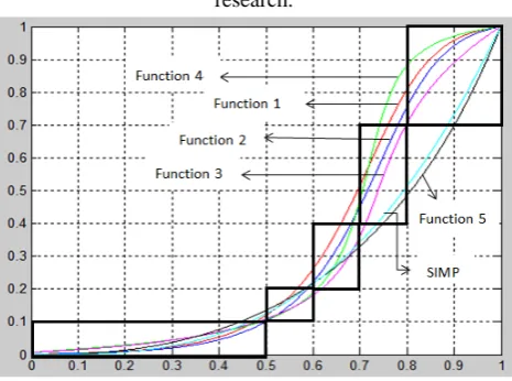
iequals 0, but they will be very close to zero. This is also necessary to prevent from forming a singular stiffness matrix of the design space. Fig. 1 shows the [image:2.595.311.544.131.304.2]SIMP function and the five functions developed in this research.
Fig. 1 SIMP and five newly developed functions of Young’s modulus
In Fig. 1, the horizontal axis represents the design variable value from 0 to 1 and the vertical axis is the value of normalized Young’s modulusE/E0. Function 5 is very similar to SIMP function. Other functions are apparently different from SIMP function, especially when design variable is greater than 0.7. The reason for developing these functions is to accelerate the design variable to reach 1 when it is already greater than 0.7. This may shorten the convergence time. The five rectangular black boxes shown in Fig. 1 are used to judge whether a developed function will be a good function that would generate a usable topology in the design space. If a function developed passes the five areas at the most of the time, there is a better chance of getting a good topology. This experience is obtained by numerous numerical simulations in this research.
B. Elimination of Checkerboard Structures
Some checkerboard eliminating methods have been developed as mentioned in the previous section. The easiest one may be the one developed by Li et al. [11].The basic idea of the method is to smooth the neighboring design variable values by using (8).
∑
∑
= = = 9 1 9 1 i i i i i i i e v w x v wx (8)
Where
x
eis the newly calculated design variable value in the center of Fig. 2,w
iis a weighting factor given in Fig. 2,i
v
is the volume of the elements,x
iis the current design variable value.It can be seen that the newly obtained design variable value is a weighted average of the design variables of the neighboring eight elements in a 2-D design space. The purpose of doing this is to reduce the big difference of design variables existing in the already formed checkerboard structure between neighboring elements. After several continuing iterations of applying this smoothing process, the black and white elements that formed the checkerboard structures will be gradually separated to disintegrate the checkerboard structure.
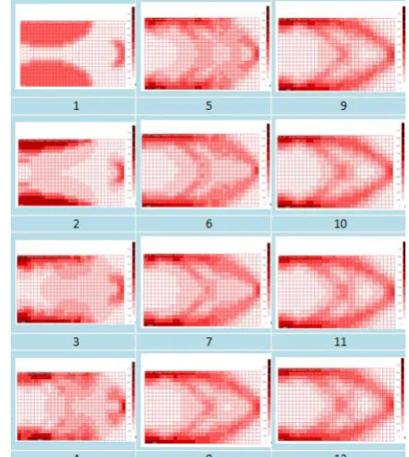
Although the purpose of eliminating checkerboard structures can be achieved by this approach, it also generates many gray elements and slows down the convergence rate. In order to eliminate checkerboard structures and also maintain the computational efficiency, the timing of adding and ending the mechanism of checkerboard elimination becomes important. This research tries to find the appropriate time period to employ the checkerboard elimination technique. Fig. 3 shows the topology variations for a problem in the first 12 iterations with checkerboard elimination technique. The problem is the most popular example used in topology optimization. It is a 2-D design space which is subjected to a concentrated load at the middle of the right hand of the design space while the structure is supported at the left hand side of the design space. The objective is to minimize the compliance and subjected to a given amount of material usage in the design space. It can be seen that the checkerboard structure appears in the early iterations and then disappears gradually from the 6th iteration. Until the 10th iteration, most checkerboard structures have gone. It is also noted that the number of gray elements is apparently large when checkerboard structures exist.
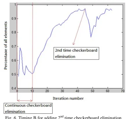
In order to understand the variations of the numbers of black and white elements during the iteration process, four curves are plotted in Fig. 4. Curve A represents the percentage of elements with design variables greater than 0.8 and less than 0.2. The larger the percentage is, the less the gray elements. Curve B shows the percentage of elements with design variable less than 0.1. Curve C is the percentage of elements with design variable greater than 0.5. Curve D is the sum of Curve B and Curve C. Fig. 4 represents a typical variation of black and white elements for some test problems. In general, the values of curves increase to a peak point first and then drop to a valley. After passing the valley point, they increase again and gradually stabilize. Observing the topologies formed in Fig. 3, a relatively clearer topology will appear at the peak point of the second increase of the curves. This timing can be used to terminate the checkerboard elimination process. However, the checkerboard structures may appear again after several iterations. Therefore, this research suggests implementing a second time checkerboard elimination at two different timings. These two timings are called timing A and timing B. For timing A, the checkerboard elimination mechanism is applied once again when Curve A reaches 75% as indicated in Fig. 5. For timing B, the checkerboard elimination mechanism is applied once again at the end of the optimization search as shown in Fig. 6. The optimization process then continues until the convergence is attained.
It is apparent from the two figures that when adding
[image:3.595.315.544.126.382.2]checkerboard elimination mechanism again, the number of black and white elements drops drastically. This seriously delays the convergence of the search process. Therefore, the checkerboard elimination mechanism should not be continuously used during the whole optimization search process.
[image:3.595.337.522.416.753.2]Fig. 3 Checkerboard structures disappearing process using (8)
Fig. 4 Variations of black and white elements
[image:3.595.340.523.578.762.2]Fig. 6 Timing B for adding 2nd time checkerboard elimination
C. Elimination of Gray Elements
Because the design variables are continuous variables varying from 0 to 1, although some penalty has been imbedded in (2) through (7), some design variables may still have values not exactly equal to 0 or 1. These elements are called gray elements. The existence of gray elements in the final topology may cause confusion to identify the true optimum topology. Therefore, some artificial steps are proposed in this research to gradually and completely eliminate gray elements in three stages. These stages are introduced as follows. Fig. 7 shows the timings of applying the 3 stages of gray element elimination mechanism.
Stage 1: Upon finishing the first time of checkerboard elimination, if Curve A increases for three consecutive iterations, the design variables greater than 0.9 are manually set to 1 and those less than 0.1 are set to 0.
Stage 2: In stage 1, only those elements that are very close to 1 or 0 are treated manually. In this stage, when Curve A stabilizes or reaches 90%, the design variables which are less than 0.3 are set to 0. The material released by these elements can be used to increase the design variables whose values are near 1 by the optimization solver automatically.
Stage 3: At the end of optimization process, there may still be a small number of gray elements. These design variables are put into an ascending order. The smallest ones are set to zero and their values are added to the largest ones to make them equal to 1. In the meantime, the satisfaction of material constraint is checked and maintained.
Fig. 7 Timings for applying elimination of gray elements
III. NUMERICAL EXAMPLE AND RESULTS
Due to limited space allowed, only one widely used example problem is given in this paper to demonstrate the results obtained from the ideas of this research. In order to understand the effects of different functions of Young’s modulus and timings on checkerboard elimination and gray element elimination, six methods are proposed. The solver used to solve the topology optimization problems is the sequential linear programming (SLP) written by the authors. Method 1: Solve the problem using SLP only.
Method 2: Solve the problem using SLP and the three stages of gray element elimination.
Method 3: Solve the problem using SLP and timing A checkerboard elimination.
Method 4: Solve the problem using method 2 and method 3 simultaneously.
Method 5: Solve the problem using SLP and timing B checkerboard elimination.
Method 6: Solve the problem using method 5 and add gray element elimination mechanism at the 2nd stage SLP searches. Example
[image:4.595.78.261.626.771.2]This example is the one used in section B. The purpose is to generate a minimum compliance topology in the 2-D design space shown in Fig. 8. The structure takes an external load acting downward at the middle of the right hand side boundary and is supported at the left hand side of the boundary. The material constraint is 25% of the total elements in the whole design space. The number of quadrilateral finite elements created in the design space is 640(32x20). Fig. 8 shows the design space and other data used for the problem.
Fig. 8 The design space and loading for the example
Fig. 9 depicts the topologies obtained by SIMP and the other five functions developed in this research. Neither mechanism of checkerboard elimination nor gray element elimination is used.
Fig. 9 Topologies obtained from different Young’s modulus functions
[image:5.595.47.292.61.238.2]The results shown in Fig. 10 through Fig. 15 are obtained from SIMP function and the other five developed functions using the six methods proposed, respectively. The different topologies in each figure are resulted from adding or without adding mechanisms of checkerboard elimination and gray element elimination using the proposed six methods for different functions of Young’s modulus. All these problems are solved by SLP with 0.25 as the initial value for all design variables. In addition to the topologies shown, the number of iterations and the compliance of the structure are listed for discussions at the end of this section.
Fig. 10 Topologies obtained by SIMP function
Fig. 11 Topologies obtained by function 1
[image:5.595.306.549.254.425.2]Fig. 12 Topologies obtained by function 2
[image:5.595.48.289.409.578.2]Fig. 13 Topologies obtained by function 3
Fig. 14 Topologies obtained by function 4
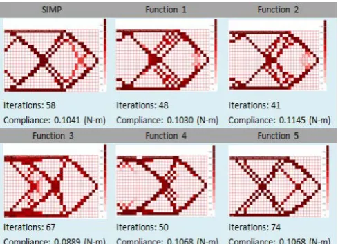
[image:5.595.48.290.599.770.2]From these figures, it can be seen that the topologies obtained have minor difference by using different functions and methods. In general, the topologies obtained by method 1 are the worst ones as expected because there is no any measure taken to prevent the forming of checkerboard structures and eliminate gray elements. Methods 2 and 4 converge much faster than other methods for all functions. The iterations spent in methods 5 and 6 are apparently greater than those for other methods as expected due to two stages of SLP searches. The topologies obtained from method 3 still yield a large area of checkerboard structures for SIMP function and function 3. This result indicates that using checkerboard elimination mechanism only may not be able to achieve its goal to eliminate checkerboard structures completely for some functions or problems. Topologies obtained from methods 2, 4 and 6 indeed are clearer than those from other methods. This proves that the gray element elimination mechanism works well. Comparing the compliance obtained from clear topologies by using methods 2, 4 and 6, the smallest compliance is 0.0905 N-m from function 3 and method 4. The second smallest compliance is 0.0938 N-m from function 4 and method 4. The compliance from SIMP function is 0.0984 N-m by method 4, but two areas of checkerboard structures are observed.
IV. CONCLUSION
Based on the results from several test problems, although not shown in this paper, the conclusion is summarized as follows.
1.Adding the mechanisms of checkerboard elimination and gray element elimination can improve the quality of topologies obtained significantly.
2.Using checkerboard elimination mechanism only may not be able to eliminate checkerboard structures completely unless it is applied in the whole optimization process. But this slows down the convergence rate.
3.Using the mechanisms of checkerboard elimination and gray element elimination simultaneously can get better quality of topologies.
4. Incorporation of Function 4 and method 4 is the best choice in terms of no checkerboard structures, clarity of topology, and computational efficiency.
REFERENCES
[1] M. P. Bendsoe and N. Kikuchi, “Generating optimal topologies in structural design using a homogenization method,” Computer Methods in Applied Mechanics and Engineering, vol. 71, pp. 197-224, 1988. [2] M. P. Bendsoe, “Optimal shape design as a material distribution
parameter problem,” Struct. Optim., vol. 1, pp. 193-202, 1989. [3] M. Zhou and G. I. N. Rozvany, “The COC algorithm, part II:
topological, geometrical and generalized shape optimization,” Computer Methods in Applied Mechanics and Engineering, vol. 89, pp. 309-336, 1991.
[4] A. R. Diaz and O. Sigmund, “Checkerboard patterns in layout optimization,” Structural Optimization, vol. 10, pp. 40-45, 2001. [5] L. Ambrosio and G. Buttazzo, “An optimal design problem with
perimeter penalization,” Calc. Var. vol. 1 pp. 55-69, 1993.
[6] R. B. Haber, M. P. Bendsoe and C. Jog, “A new approach to variable topology shape design using a constraint on the perimeter,” Struct. Optim., vol. 11, pp. 1-12, 1996.
[7] J. Ptersson and O. Sigmund, “Shape constrained topology optimization,” Int. J. Numer. Meth. Engrg. vol. 41, pp. 1417-1434, 1998.
[8] O. Sigmund and J. Petersson, “Numerical instabilities in topology optimization: A survey on procedures dealing with checkerboards,
mesh-dependencies and local minima,” Strut. Optim., vol. 16, pp. 68-75, 1998.
[9] M. Zhou, Y. K. Shyy and H.L. Thomas, “Checkerboard and minimum member size control in topology optimization,” Struct. Optim., vol. 21, pp. 152-158, 2001.
[10] Y. Du and D. Chen, “Suppressing gray-elements in topology optimization of continua using modified optimality criterion methods,” CMES, vol. 86, no. 1, pp. 53-70, 2012.