The First Order Autoregressive Model with Coefficient
Contains Non-Negative Random Elements: Simulation
and Esimation
Pham Van Khanh
Military Technical Academy, Hanoi, Vietnam Email: [email protected]
Received October 14,2012; revised November 14, 2012; accepted November 27, 2012
ABSTRACT
This paper considered an autoregressive time series where the slope contains random components with non-negative values. The authors determine the stationary condition of the series to estimate its parameters by the quasi-maximum likelihood method. The authors also simulate and estimate the coefficients of the simulation chain. In this paper, we consider modeling and forecasting gold chain on the free market in Hanoi, Vietnam.
Keywords: Random Coefficient Autoregressive Model; Quasi-Maximum Likelihood; Consistency
log max log ,0
1. Introduction
x x .It is well-known that many time series in finance such as stock returns exhibit leptokurtosis, time-varying volati- lity and volatility clusters. The generalized autoregres- sive conditional heteroscedasticity (GARCH) and the ran- dom coefficient autoregressive (RCA) model have been caturing three characteristics of financial returns.
The RCA models have been studied by several authors [1-3]. Most of their theoreic properties are well-known, including conditions for the existence and the uniqueness of a stationary solution, or for the existence of moments for the stationary distribution. In this paper, we address the stationary conditions for the RCA model, the exis- tence and the uniqueness of a stationary solution and parameter estimation problem for the RCA model with the coefficient have a non-negative random elements.
2. Stationary Conditions of the Series
Consider time series
Yt satisfying
0,
,t t
t e
Y b
e N
1
2 0, 2
t t
t b
Y e
b N
(1) where
b e,
,,P
t t t z are random vectors with independent
identical distribution defined in a certain
probability space (2) Firstly, we consider the property of the stochastic vari- able
1
0 i
i j
j
b
0 i
Y e
(3)Let
Lemma 1. Suppose that condition (2) satisfied,
0 0
log and log
E e E b (4) If
0
log 0
E b (5)
Y determined by (3) will be absolute convergence with probability 1.
Proof.
Assume Elogb0 0
0
, according to the law of great numbers, existing stochastic variable i such that:
1 2
0
1
log log log
2 with every
i
b b b i
i i
(6)
0
log 0
E b
where . Then
0
0 0
0
1 1
0 0 1 0
1
/ 2
0 0 1
i i i
i j i k
i j i i k
i i
i
i j i
i j i i
Y e b e b
e b e e
(7)
We will prove 2
0
1
i i i
P e e
. Indeed, due to2
0 i 1
e a
nd in accordance with lemma Borel-Cante- lli, sufficient condition here means proving
1
k k k
P e
1 1
1
0
log
log
log log
k
k k
k
P e P
P e
E e
0
log
log
.
k ek k
k
From (7), we have P Y
1.If 0
0
log
E b , (6) can always correct with some . Therefore, (7) is always true.
Lemma 2. Suppose that (2) and (5) meet
0 and 0 with some
E b E e 0
0
. Then, existing such that E Y .
Proof.
Suppose
0 ,0t
M t E b t
0 1M
We have , and owing to 5 :M
0 0,
M t is a decreasing function in the neighborhood of 0.
Hence, existing 0 M
1 .such that . Generally less, suppose that 0 1
b
Due to the convex, we have
ab
a với a b, 0.1
0
.
i j
i j
b
e b
0 1
0 0
i
i j
i
i j
Y e
1M
Use condition (2) and , we obtain:
1
0
.
i
j j
i b 0
0
0 0 i
i
E Y E e E
E e M
Lemma 3. Assume (2) and (5) are satisfied with
0 0
1:E e ,E b and
E b0 1
. Then
E Y . Proof.
Due to condition (2) and inequality Minkowski
1
1
0
0 i
E Y E e E
b0 i
. Hence, E Y .
Theorem 1: Suppose that (1), (4) and (5) satisfied
with the almost sure convergence of
10 i bk
Yk;kZY
j
0 i
k k
i j
Y e
and process
isthe stationary solution of (1)
Proof.
k is convergent absolutely, acording to Lemma 1
We have: 1
0 i
i k j
j b
0
k k
i
Y e
. Therefore:
1
1 0
1 2 1
1 1
1
1 1
0 0
1 i
k k k i k j
i j
k k k k k k
k m k k k m
i
k k k i k j
i j
k k k
Y e e b
e e b e b b
e b b b
e b e b
e b Y
Y
k
Obviously,
is the single solution of (1)
Yk is a stationary series and
Yk, ,
t t e b tk
is independent of .
3. Estimation of Model Parameters
Suppose that
0 0
2
0 0 2
2 2
, 0, 0 ;
0
cov , ,
0
0, 0.
b
e
b e
E b e
b e
In this section, we care about estimating vectors of
, 2, 2
b e
Z k
based on Quasi-Maximum Likelihood method.
, we have: With
1 1 1
1
k k k k k k
k k
E Y E b Y e
E b Y
2
π
k b
E b
but , so
1 1
2
1 1 1
2
2 2
1 1
2 2 2
1
2 2 2 1
2
π
2 Var
π
2
π
2 2
1 2
π π
2
1 .
π
k k b k
k k k b k k
k b k k k
b b k k e
b k e
E Y Y
Y E Y Y
E b Y e
E b Y
Y
1
2π 1
2 π 1 exp 2 2 1 π n n i L u 2 1 2 1 2 1 1 2 π . i i i i xY y x Y y
ˆn n n
L u L
Y s xY
Maximum likelihood estimators determined by:
sup n 3 R (8) where is a certain optional appropriate area of
Let
1 1 2 1 π log 1 n n i i iH u g
n Y s g u 2 1 2 1 2 1 2 π 2 . π i i i i u x Y xY y xY y
ˆn n n
H u H
Then (8) can be written as inf
n
Assume
0 00 0 0
, , : , ,
with 0, 1, 1
0 0
0 0
1 1
s x y s s s x x
s x y
y y x y ˆ (9)
Now, the consistence of maximum livelihood esti- mates n is said.
Theorem 2. Suppose (2), (4), (5), (8), (9) satisfied and
0 0
P b e
ˆ a.s n
0 1 and
. We have
n .
Proof.
Let
11
2 1
, , , 0,1
2 1 π i i i Y Y u xY y
, , 2 , N
and
02 0 , , 2 1 π Y E xY y
0,1, , 2 .
1 and Eg u1
We will prove inf
be con-u
E g u
tinuous on .
Indeed,
2 0 2 0 2 0 0 00 0 0 2 1 0 1 2 0 2 0 2 sup log 1
π
2 1
1 2
π
log log 1
π log 2 π inf inf 2 1 π 2
sup log 1
π u
u u
E xY y
Y
E E x Y y
x y
y
Y s x Y
E g u E
xY y
E xY y
2 1 0 2 0 2 0 2 π inf 2 1 π 2 sup log 1
π u
u
Y s x Y
E
xY y
E xY y
On the other hand,
2 1 0 1 2 0 2 0 2 π 2 1 π 2 log 1 π
Y s x Y
Eg u E
xY y
E xY y
But
2 1 0 22 2 2
0 1 0
2 2 1 0 2 π 2 1 π 2 2 π e
Y s x Y
Y b x Y
x
s b Y
2 2 1 12 2 4
π π π
2 2
π π
b b
b x
E b x x
x
E b x
2 0 1 2 0 2 2 2 2 0 2 0 2 1 π 42 2 2
π π π
2 log 1 2 π 1 π b b b e Y Eg u E
xY y
x x
s x s
xY y
1 Eg u
, ,
u s x y
0,u u
E E xY y
is a continuous function in acordance with . Next, we will prove:
1 1
Eg u Eg .
In fact,
2 0 1 2 0 2 2 2 2 0 2 0 2 2 0 2 02 2 2 0
2 1
π
4
2 2 2
π π π
2 log 1 2 π 1 π 2 2 π 1 π 2 1 π 2 1 π b b e b b e Y Eg u E
xY y
x x
b
s x s
xY y E E xY y Y
s x E
xY y Y E
2 2 0 2 2 0 02 2 2 0
2 2
0
2 0
2 2 2 0 2 0 2 1 π log 2 1 π 2 log 1 π 2 2 π 1 π 2 1 2
π log 1
2 π 1 π b b e b b e Y E
xY y Y
E Y
Y
s x E
xY Y Eh E xY y 2 2
2 2 2 0 b e b e y y Y
( )
( )
( )
( )
( )
( )
( )
1 1ln , 0 1
1 , 0 1
1 1 0
h x x x x
h x h x x
x
h x h x
Eg u Eg q
= - >
¢ = - ¢ = =
> = " >
³
where
1 1
Eg u Eg
and if and only if
2 2 2 0 2 0 2 2 2 1
2 0 and 1π 1
2 π 1 π , , b e b b e Y
s x P
xY y
x y s
If
2 2 2 2
0 0
2 2 2
0 2 2 1 1 π π 2 1 π b e b e
Y xY y a.s
x Y y a.s
2 b ,
If x or ye2, P Y
02c
1
But 2 2 2
1 1 0 1 2 1 1 0 .
Y b Y e b e Y a s
Y kk, Z
is a stationary seriesBut
2 1 21 1 1 1 0
1
2 .
P Y c
c b c e b e Y a s
0
EY
But 0 , take conditional expectations e b1, 1
in both sides, we have:
2
1 1 .
c b ce a s But Y0 c a s.
b1
e10 .a s
inf n n
u l u l
Return to theorem
, so
lim supinf n lim sup n . .
n ul u n l a s
gi ,
But series iZ is stationary and ergodic with E g1
, according to Ergodic theorem, wehave:
1
1
lim .
lim supinf .
n n
n
n u
l Eg a s
l u Eg a s
,n n l u
With each positive integer is a continuous function in compact set G, so
1
ˆ lim sup .
n n n
n l Eg a s
C
Let -compact set in with positive distance to
. Owing to g1(u) being continuous in , existing an
open sphere U(u) with center u with
such that:
1
inf
t U u
r E g t
,U u uC
, , ,U u
1 j k
.
Sets are open covers of C, so C holds such finite open covers, are called
1 2 k of C. In accordance with
Er-godic thoerem, with every
, we have:U u U u
1
1
lim inf inf
j j
n
i
n i u U u u U u 1
.
g u E
n
g u r a sSee that
inf
inf
j j
j
i U u
n i
u g u
g u r
0
r
1
inf
u C
r E
1
f .
u CEg u a s
Eg u C
1 1 1
1 1
1
inf min inf min
1
lim inf inf min lim inf
n
n n
u C j ku U u j k i u
n
n u C j k n i u U
l u l u
n
l u
n
In out of events Br with with satis-
g u
r P Bfying: .
Therefore, lim inf inf n
inn u C l u
But 1 is continuous and
1 Eg u
1 . Eg a s
is singly minimum of
lim inf inf n n u C l u
Let U is a open sphere with center and enough small radius and U U . If n , existing a
random subseries n such that with
ˆ U
k
C , we
have:
U
ˆ m inf k kn ln n
s
*
lim inf inf li lim sup .
n u C k
n n n
l u
l a
inf inf n u C l u
0
, .
U n n
, 2, 2
But lim sup n
ˆn 1
lim n l Eg n
hence, with each above U , existing random variable such that
0
n ˆn
This completes the proof.
4. Simulation
In this section, we simulate series (1) with different val- ues of b e
, 2, 2
. These simulations show station- ary and non-stationary series cases.
We simulate series (1) with different values of
[image:5.595.311.536.86.213.2]b e
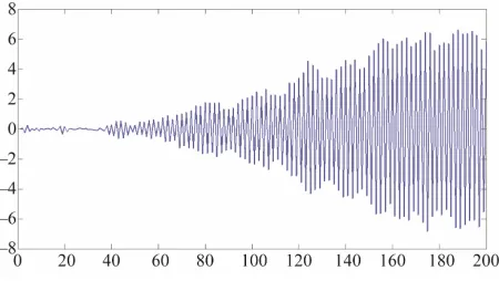
Figure 1. Simulation for series Yt defined by (1) with
. 1.09;σb 0.1;σe 0.1
[image:5.595.313.536.257.384.2]
Figure 2. Simulation for series Yt defined by (1) with
. .9;σb 0.1;σe 0.1
[image:5.595.310.536.421.543.2]
Figure 3. Simulation for series Yt defined by (1) with
.93;σb 0.1;σe 0.1
.
1.07
and in each case we can check the sta- tionary conditions of the series(1) by Lemma 1. In Fig-
ure 1, we see that the series is not stationary with the
negagtive slope and in Figures 2 and 3 we
simulate the not stationary series with positive slope 0.9
and 0.93 0.7
. Figure 4 presents astationary but
clustering series, Figures 5-7 presentstationary series with
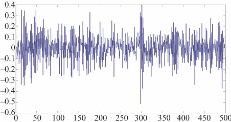
[image:5.595.310.537.585.706.2]Figure 8. Return series of Gold price rt.
Figure 5. Simulation for series Yt defined by (1) with
.7;σb 0.1;σe 0.1
[image:6.595.58.286.250.368.2] .
Figure 9. Simulation for series Yt defined by (1) with
ˆ 0.0004,0.0002,0.0069
θ .
Figure 6. Simulation for series Yt defined by (1) with
. ;
[image:6.595.58.287.415.532.2] σb0.1;σe0.1
Figure 9 below is a simulation of the process (1) with
parameters ˆ
0.0004,0.0002,0.0069
.6. Conclusion
This paper has solved some problems relating to a kind of first order time series with coefficient regression af- fected by non-negative random elements. In subsequent studies, the author will consider the asymptotic estimates of the parameters.
REFERENCES
Figure 7. Simulation for series Yt defined by (1) with.7; [1] T. Bollerslev, “Generalized Autoregressive Conditional Heteroscedasticity,” Journal of Econometrics, Vol. 31, No. 3, 1986, pp. 307-327.
doi:10.1016/0304-4076(86)90063-1
0.1; 0.1
b e
σ σ
t
r
.
5. Application for Real-Time Series
[2] D. Nicholls and B. Quinn, “Random Coefficient Autore- gressive Models: An Introduction,” Springer, New York, 1982. doi:10.1007/978-1-4684-6273-9
In this section, we use model (1) for the model of return series of the price of gold on the free market in Hanoi, Vietnam. Figure 8 show the Return series of Gold price
.
From the data series we estimate for vector
, 2, 2
b e
is ˆ
0.0004,0.0002,0.0069
. So, we[3] A. Aue, L. Horvath and J. Steinbach, “Estimation in Random Coefficient Autoregressive Models,” Jour- nal of Time Series Analysis, Vol. 27, No. 1, 2006, pp. 61-76. doi:10.1111/j.1467-9892.2005.00453.x
can use the following model to forecast the future value of gold price:
1
0.0004 0,0.0069 ,
t t
t t
r b
e N b
0,0.0002 .
t t
r e
N