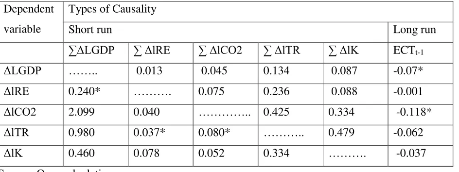
Does renewable energy consumption drive economic growth: Evidence from Granger causality technique
Full text
Figure
Related documents
In the current classification of pulmonary hypertension (PH) ( table 1 ), PAH is defined as ‘‘group 1’’ and can be idiopathic, heritable or associated with different
Since borrowers are typically willing and able to borrow more at lower prices, the demand curve slopes down and to the right, illustrating that higher prices, in this case
Zheng Zhang et al.’s [5] method employed vertical projection to recover document images that contain marginal noise, and decided whether the marginal noise was
The intrinsic failure is caused by actual defects in products, the marginal failure is a decisive problem of devices of which quality is on the border of non-defective
Frontier analysis – like Data Envelopment Analysis – is a powerful method for efficiency measurement, whereas BPS has shown to be successful in analyzing the structure of
Dr. HANCOCK said theie were several matters in Mr. Heron's paper that required notice. Hancock's) report he stated, after careful inquiry, that there were no official returns of
Based on Socio-economic, Political and cultural heritage of the country. Education System of the global perspective was taken into consideration. The report
