Munich Personal RePEc Archive
Measuring the Distributions of Public
Inflation Perceptions and Expectations in
the UK
Murasawa, Yasutomo
Faculty of Economics, Konan University
16 January 2017
Online at
https://mpra.ub.uni-muenchen.de/76244/
MEASURING THE DISTRIBUTIONS OF PUBLIC
INFLATION PERCEPTIONS AND EXPECTATIONS IN
THE UK
∗YASUTOMO MURASAWA†
Faculty of Economics, Konan University, Kobe, Japan
January 16, 2017
SUMMARY
The Bank of England/GfK NOP Inflation Attitudes Survey asks individuals about their inflation perceptions and expectations in eight ordered categories with known boundaries except for an indifference limen. With enough categories for identification, one can fit a mixture distribution to such data, which can be multi-modal. Thus Bayesian analysis of a normal mixture model for interval data with an indifference limen is of interest. This paper applies the No-U-Turn Sampler (NUTS) for Bayesian computation, and estimates the distributions of public inflation perceptions and ex-pectations in the UK during 2001Q1–2015Q4. The estimated means are useful for measuring information rigidity.
Keywords Bayesian, Indifference limen, Information rigidity, Interval data, Normal mix-ture, No-U-turn sampler
JEL classification C11, C25, C46, C82, E31
∗This work was supported by JSPS KAKENHI Grant Number 16K03605.
†Correspondence to: Yasutomo Murasawa, Faculty of Economics, Konan University, 8-9-1 Okamoto,
Higashinada-ku, Kobe, Hyogo 658-8501, Japan.
1
INTRODUCTION
Inflation (or deflation) and its expectations both play important roles in macro and mon-etary economics. Prices move differently across regions and commodities. Since people live in different regions and buy different commodities, they perceive inflation and form its expectations in different ways, even if they are fully rational. Perhaps people are boundedly rational in different ways, or may be irrational. Whatever the reason is, survey data on inflation perceptions and expectations show substantial heterogeneity or disagree-ment among individuals that varies over time with the actual inflation; see Mankiw et al. (2004). It is thus of interest to central banks to monitor not only the means or medians of the actual, perceived, and expected inflation but also their whole distributions among individuals. Indeed, the mean, median, and mode may be quite different.
Survey questions often ask respondents to choose from more than two categories. The categories may be ordered or unordered, and if ordered, they may or may not represent intervals. Thus there are three types of categorical data: unordered, ordered, and interval data. Interval data have quantitative information.1 To analyze these data (with
covari-ates), we use multinomial response, ordered response, and interval regression models for unordered, ordered, and interval data respectively.2
Some categorical data are not exactly one of the three types but somewhere in between. For a question asking about a change of some continuous variable with several intervals to choose from, there is often a category ‘no change.’ This does not literally mean a 0% change, whose probability is 0, but corresponds to anindifference limen, which allows for a very small change. Data on inflation perceptions and expectations are examples. The problem is that we do not know the boundaries of an indifference limen.
A simple solution is to combine an indifference limen with its neighboring intervals to apply interval regression. Alternatively, one may assume a common indifference limen among individuals. Then assuming a parametric distribution for the latent continuous variable, with enough categories for identification, one can estimate the distribution
pa-1
Interval data lose some quantitative information, however. If the first or last interval has an open end, then one cannot draw a histogram nor compute its mean. Moreover, one cannot find the median if it lies in the first or last interval with an open end. To solve the problem, one can assume the minimum or maximum of the population distribution, or fit a parametric distribution to the frequency distribution.
2
rameters and the common indifference limen jointly. Given the prior information that the indifference limen contains 0 and cannot overlap with the other intervals, this may improve efficiency. Murasawa (2013) applies these ideas to survey data on inflation expec-tations. This paper complements Murasawa (2013) in three ways: data, distribution, and methodology.
First, Murasawa (2013) uses monthly aggregate interval data on household inflation expectations in Japan during 2004M4–2011M3 that have seven intervals lying symmet-rically around 0. This paper uses quarterly aggregate interval data on public inflation perceptions and expectations in the UK during 2001Q1–2015Q4 that have eight intervals, six of which lie above 0. Thus we can compare the distributions of inflation expectations and their dynamics in Japan and the UK, if desired. Moreover, the UK data allow us to study the interaction between inflation perceptions and expectations.
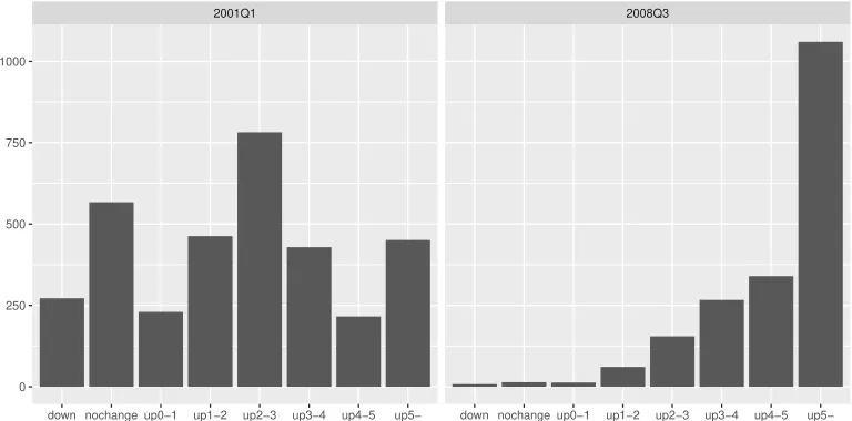
Second, Murasawa (2013) considers normal, skew normal, skew exponential power, and skew t distributions, which are all unimodal and have at most four parameters. Since the UK data have one more interval, this paper considers a mixture of two normal distribu-tions, which can be bimodal with five parameters. The frequency distributions of the UK data may have two modes; see the left panel in Figure 1.3 Hence mixture distributions may fit better than unimodal skew distributions. Even if not, one cannot exclude multi-modal distributions a priori.
(Figure 1)
Third, Murasawa (2013) applies the ML method. The likelihood function of a normal mixture model for numerical data is unbounded, however, when one component has mean equal to a data point and variance equal to 0; see Kiefer & Wolfowitz (1956, p. 905). The likelihood function is bounded for interval data, but Biernacki (2007) shows that the global ML estimate may still have a degenerate component or otherwise the EM algorithm may converge to a local ML estimate with a degenerate component. To avoid the problem, this paper applies Bayesian analysis. MCMC methods are useful for posterior simulation. With an indifference limen, our model is similar to an ordered response model, for which the Gibbs sampler and M–H algorithm are often slow to converge for large samples. Instead,
3
this paper applies a Hamiltonian Monte Carlo (HMC) method, in particular the No-U-Turn Sampler (NUTS) developed by Hoffman & Gelman (2014).
Because of the label switching problem, MCMC methods may not work for the compo-nent parameters of a finite mixture model. It works for permutation invariant parameters, e.g., moments and quantiles, however; see Geweke (2007). We analyze three types of data, and find the following:
1. With six intervals ignoring the indifference limen, the estimated means are reason-ably precise. However, the estimates of higher order moments are often imprecise with wide error bands. This tends to occur when the majority of the respondents choose the last interval with an open end; see the right panel in Figure 1.
2. With eight intervals including the indifference limen and the prior information that the indifference limen contains 0, the results change slightly, especially for higher order moments. However, the estimated distributions are not precise enough to learn about the dynamics of the distributions of inflation perceptions and expectations. The estimated indifference limens are time-varying and often strongly asymmetric around 0. In particular, the estimated lower bounds of the indifference limens are often far below −1.0%.4
3. Data with 18 intervals are available since 2011Q2, which often have two more local modes at ‘Up by 7% but less than 8%’ and ‘Down by 1% but less than 2%’ (or ‘Down by 2% but less than 3%’); see Figure 2. If we fit a mixture of two normal distributions to these data, then the estimated distributions and indifference limens seem precise.5 With only 19 quarters of samples (2011Q2–2015Q4) covering at most one business cycle, though, we cannot learn much about the dynamics of the distributions of inflation perceptions and expectations.
Thus we find that fitting flexible distributions to repeated interval data requires well-designed categories to provide enough information about the shapes of the underlying distributions, which may shift drastically over time. The problem exists but is much
4
If this makes no sense, then one can impose a subjective prior for the lower bound of the indifference limen, which will change the results further.
5
less evident when fitting normal or unimodal distributions. This consideration seems important when designing a repeated survey.6
(Figure 2)
This paper contributes to the literature on quantification of qualitative survey data in three ways. First, we propose a normal mixture model for interval data with an indifference limen. This seems new, and its flexibility seems useful for analysis of survey data. Second, we propose Bayesian analysis of the model using the NUTS. This is useful since for this model, ML estimation may fail, and the Gibbs sampler and M–H algorithm are often slow to converge for large samples. Third, we apply the method to survey data on inflation perceptions and expectations in the UK repeatedly, and estimate their distributions during 2001Q1–2015Q4.
To illustrate a possible use of the estimated distributions, we measure the degrees of information rigidity in public inflation perceptions and expectations in the UK using a simple framework proposed by Coibion & Gorodnichenko (2015), which requires only the historical means of the distributions of expectations. We find some evidences of infor-mation rigidity, but the results depend on what prices we assume individuals forecast, i.e., the CPI or RPI, and how we estimate the distributions of inflation perceptions and expectations, i.e., the choice of the number of mixture components and whether to include or exclude the indifference limen.
The paper proceeds as follows. Section 2 reviews some relevant works. Section 3 specifies a normal mixture model for interval data with an indifference limen. Section 4 specifies our prior, and explains our posterior simulation. Section 5 applies the method to aggregate interval data on public inflation perceptions and expectations in the UK during 2001Q1–2015Q4. Section 6 measures information rigidity in public inflation perceptions and expectations in the UK during 2001Q1–2015Q4. Section 7 concludes with discussion.
6
2
LITERATURE
2.1 Quantification of Qualitative Survey Data
This paper contributes to the literature on quantification of qualitative survey data, in particular the Carlson–Parkin (C–P) method; see Nardo (2003) and Pesaran & Weale (2006, sec. 3) for surveys. To quantify ordered data, which have no quantitative informa-tion, the C–P method requires multiple samples and strong assumptions; i.e., normality, a time-invariant symmetric indifference limen, and long-run unbiased expectations. These assumptions often fail in practice, however; see Lahiri & Zhao (2015) for a recent evidence. Such strong assumptions are unnecessary for interval data, to which one can fit various distributions each sample separately. Using aggregate interval data from the Monthly Consumer Confidence Survey in Japan, Murasawa (2013) fits various skew distributions by the ML method, which also gives an estimate of the indifference limen. Using the same data and approximating the population distribution up to the fourth cumulant by the Cornish–Fisher expansion, Terai (2010) estimates the distribution parameters by the method of moment.
2.2 Measuring Inflation Perceptions and Expectations
Empirical works on inflation perceptions and expectations are abundant; see Sinclair (2010) for a recent collection. Most previous works use either ordered or numerical data, however, since few surveys collect interval data on inflation perceptions and expectations. Exceptions are Lombardelli & Saleheen (2003) and Blanchflower & MacCoille (2009), who use individual interval data from the Bank of England/GfK NOP Inflation Attitudes Sur-vey and apply interval regression to study the determinants of public inflation expectations in the UK.
Recent works try to measure subjective pdfs of future inflation. For surveys, see Manski (2004) on measuring expectations in general and Armantier et al. (2013) on measuring inflation expectations in particular.
2.3 Bayesian Analysis of a Normal Mixture Model for Interval Data
interval data with no indifference limen. Estimation of an indifference limen is similar to estimation of cutpoints in an ordered response model and hence troublesome.
Albert & Chib (1993) develop a Gibbs sampler for Bayesian analysis of an ordered response model, but it converges slowly, especially with a large sample. To improve con-vergence, Cowles (1996) applies ‘collapsing,’ i.e., sampling the latent data and cutpoints jointly, which requires an M–H algorithm. Nandram & Chen (1996) and Chen & Dey (2000) reparametrize the cutpoints for further improvement.7 For an M–H algorithm, however, one must choose good proposals carefully, which is a difficult task. Moreover, the optimal acceptance probability may be far below 1, in which case substantial ineffi-ciency remains; see Gelman et al. (2014, p. 296).
3
MODEL SPECIFICATION
Letybe a random sample of sizentaking values on{1, . . . , J}, which indicateJ intervals onR. Assume an ordered response model foryi such that fori= 1, . . . , n,
yi:=
1 ifγ0 < y∗i ≤γ1 ..
.
J ifγJ−1 < y∗i ≤γJ
(1)
where y∗i is a latent variable underlying yi and −∞ = γ0 < · · · < γl < 0 < γu < · · · <
γJ =∞. Assume that we know {γj} except for an indifference limen [γl, γu]. Assume a normal K-mixture model foryi∗ such that fori= 1, . . . , n,
yi∗∼
K
∑
k=1
πkN(
µk, σ2k
)
(2)
Let π := (π1, . . . , πK)′, µ := (µ1, . . . , µK)′, σ := (σ1, . . . , σK)′, γ := (γl, γu)′, and θ := (π′,µ′,σ′,γ′)′. Assume for identification that π1 ≥ · · · ≥ πK. Consider estimation of θ giveny.
7
4
BAYESIAN ANALYSIS
4.1 Prior
For mixture models, independent improper priors on the component parameters give im-proper posteriors if some components have no observation. Instead, we useweakly infor-mative priors in the sense of Gelman et al. (2014, p. 55).
For the mixture weight vector π, we assume a Dirichlet prior such that
π|µ,σ,γ ∼D(ν0) (3)
Settingν0:=ıKgives a flat prior on the unit (K−1)-simplex. We impose the identification restrictionπ1 ≥ · · · ≥πK after posterior simulation by relabeling, if necessary.
For the component meansµ1, . . . , µKand variancesσ12, . . . , σK2 , we assume independent normal–gamma priors such that fork= 1, . . . , K,
µk|µ−k,σ,π,γ∼N
(
µ0, σ20 )
(4)
σ2k|σ−k,µ,π,γ∼Inv-Gam(α0, β0) (5)
Setting a largeσ0gives a weakly informative prior onµ1, . . . , µK. The prior onσ21, . . . , σK2 implies that fork, l= 1, . . . , K such thatk̸=l,
σk2
σl2|σ−(k,l),µ,π,γ ∼F(2α0,2α0) (6)
Thusα0 controls the prior on the variance ratio. To avoid the variance ratio to be too close
to 0, which avoids degenerate components, one often setsα0 ≈2; see Fr¨uhwirth-Schnatter
(2006, pp. 179–180). It is difficult to set an appropriateβ0 directly. Instead, Richardson
& Green (1997) propose a hierarchical prior onβ0 such that
β0 ∼Gam(A0, B0) (7)
Let R be the range of the sample, i.e., y∗ := (y∗
settings:
µ0 :=m (8)
σ0 :=
R
c (9)
α0 := 2 (10)
A0 :=.2 (11)
B0 :=
A0
α0
100
R2 =
10
R2 (12)
wherec >0 is a small integer.
For the boundaries of the indifference limen [γl, γu], we assume independent uniform priors such that
γl|γu,π,µ,σ∼U(λ0,0) (13)
γu|γl,π,µ,σ∼U(0, υ0) (14)
where
λ0:= max
γj<γl
{γ0, . . . , γJ} (15)
υ0:= min
γj>γu{γ0, . . . , γJ} (16)
4.2 Posterior Simulation
An MCMC method sets up a Markov chain with invariant distributionp(θ|y) for posterior simulation. After convergence, one can treat the realized states of the chain as (serially dependent) draws fromp(θ|y). Let q(θ,θ′) be a transition kernel that defines a Markov chain. A sufficient (not necessary) condition for a Markov chain to converge in distribution top(θ|y) is thatp(θ|y) andq(θ,θ′) are in detailed balance, i.e., ∀θ,θ′,
p(θ|y)q(θ,θ′) =p(θ′|y)q(θ′,θ) (17)
crucial for successful posterior simulation.
Understanding an HMC method requires some knowledge of physics. The Boltzmann (Gibbs, canonical) distribution describes the distribution of possible states in a system. Given an energy functionE(.) and the absolute temperature T, the pdf of a Boltzmann distribution is∀x,
f(x)∝exp
(
−E(x) kT
)
(18)
wherekis the Boltzmann constant. One can think of any pdff(.) as the pdf of a Boltzmann distribution withE(x) :=−lnf(x) andkT = 1.
The Hamiltonian is an energy function that sums the potential and kinetic energies of a state. An HMC method treats−lnp(θ|y) as the potential energy at positionθ, and introduces an auxiliary momentumzdrawn randomly from N(0,Σ), whose kinetic energy is−lnp(z)∝z′Σ−1z/2 with mass matrixΣ. The resulting Hamiltonian is
H(θ,z) :=−lnp(θ|y)−lnp(z)
=−lnp(θ,z|y) (19)
An HMC method draws from p(θ,z|y), which is a Boltzmann distribution with energy functionH(θ,z).
The Hamiltonian is constant over (fictitious) time t by the law of conservation of mechanical energy, i.e.,∀t∈R,
˙
H(θ(t),z(t)) = 0 (20)
or
˙
θ(t)Hθ(θ(t),z(t)) + ˙z(t)Hz(θ(t),z(t)) =0 (21)
Thus Hamilton’s equation of motion is∀t∈R,
˙
θ(t) =Hz(θ(t),z(t)) (22)
˙
z(t) =−Hθ(θ(t),z(t)) (23)
1. Drawz ∼N(0,Σ) independently fromθ.
2. Start from (θ,z) and apply Hamilton’s equations of motion for a certain length of (fictitious) time to obtain (θ′,z′), whose joint probability density equals that of (θ,z).
3. Discardz andz′, and repeat.
This gives a reversible Markov chain on (θ,z), since the Hamiltonian dynamics is re-versible; see Neal (2011, p. 116). The degree of serial dependence or speed of convergence depends on the choice of Σ and the length of (fictitious) time in the second step. The latter can be fixed or random, but cannot be adaptive if it breaks reversibility.
In practice, an HMC method approximates Hamilton’s equations of motion in discrete steps using the leapfrog method. This requires choosing a step size ϵ and the number of stepsL. Because of approximation, the Hamiltonian is no longer constant during the leapfrog method, but adding a Metropolis step after the leapfrog method keeps reversibil-ity. Thus givenΣ and an initial value forθ, an HMC method proceeds as follows:
1. Drawz ∼N(0,Σ) independently fromθ.
2. Start from (θ,z) and apply Hamilton’s equations of motion approximately by the leapfrog method to obtain (θ′,z′).
3. Accept (θ′,z′) with probability min{exp(−H(θ′,z′))/exp(−H(θ,z)),1}.8
4. Discardz andz′, and repeat.
The degree of serial dependence or speed of convergence depends on the choice of Σ, ϵ, andL. Moreover, the computational cost of each iteration depends on the choice ofϵand
L.
The NUTS developed by Hoffman & Gelman (2014) adaptively choosesLwhile keeping reversibility. Though the algorithm of the NUTS is complicated, it is easy to use with Stan, a modeling language for Bayesian computation with the NUTS (and other methods).
8
Stan tunesΣ and ϵ adaptively during warmup. The user only specifies the data, model, and prior. One can call Stan from other popular languages and softwares; e.g., R, Matlab, and Stata. The NUTS often has better convergence properties than other popular MCMC methods such as the Gibbs sampler and M–H algorithm.
5
INFLATION PERCEPTIONS AND EXPECTATIONS IN
THE UK
5.1 Data
We use aggregate interval data from the Bank of England/GfK NOP Inflation Attitudes Survey that started in February 2001.9 This is a quarterly survey of public attitudes to inflation that interviews a quota sample of adults aged 16 or over in 175 randomly selected areas throughout the UK. The quota is about 4,000 in February surveys and about 2,000 in others. Detailed survey tables are available at the website of the Bank of England. Moreover, the individual data are now publicly available.
The first two questions of the survey ask respondents about their inflation perceptions and expectations:
Q.1 Which of the options on this card best describes how prices have changed over the last twelve months?
Q.2 And how much would you expect prices in the shops generally to change over the next twelve months?
The respondents choose from the following eight intervals (excluding ‘No idea’):
1. Gone/Go down
2. Not changed/change
3. Up by 1% or less
4. Up by 1% but less than 2%
5. Up by 2% but less than 3%
9
6. Up by 3% but less than 4%
7. Up by 4% but less than 5%
8. Up by 5% or more
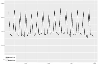
The questionnaire gives the boundaries between the categories except for category 2, which is an indifference limen.10 We exclude ‘No idea’ from the samples in the following analyses. Figure 3 plots the sample sizes for the two questions during 2001Q1–2015Q4.
(Figure 3)
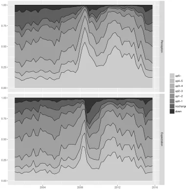
Figure 4 plots the relative frequencies of the categories for inflation perceptions and ex-pectations during 2001Q1–2015Q4. The perceptions and exex-pectations are heterogeneous, but on average, they rose in 2007, reached a peak in 2008Q3, and then dropped. They rose again in 2010, remained high for a while, and then slowly decreased toward 2015.
(Figure 4)
The relative frequency of category 3 is often lower than those of categories 2 and 4. Hence the distributions of inflation perceptions and expectations may be bimodal, depending on the interval widths of categories 2 and 3. To allow for this possibility, we fit a mixture of two normal distributions and estimate the indifference limen each quarter.
5.2 Model Specification
Our model consists of equations (1)–(2) withJ := 6 (with no indifference limen) or 8 (with an indifference limen) and K := 2. Our priors are those in section 4.1 with m := 2.5,
R:= 10, andc:= 1. Thus we setν0 :=ı2,µ0:= 2.5,σ0:= 10,α0 := 2,A0:=.2,B0:=.1,
λ0 :=−∞, andυ0 := 1. These weakly informative priors do not dominate the posteriors
for our samples.
Reparametrizatoin may improve efficiency of MCMC. Following Betancourt & Girolami (2015), one may reparametrize our hierarchical model from centered parametrization (CP)
10
to noncentered parametrization (NCP); i.e., instead of equation (5), fork= 1, . . . , K, one may draw
σ∗2k|σ−k,µ,π,γ ∼Inv-Gam(α0,1) (24)
and set σk2 := β0σ∗2k. CP and NCP are complementary in that when MCMC converges slowly with one parametrization, it converges much faster with the other parametrization; see Papaspiliopoulos et al. (2003, 2007). We find that CP is often faster than NCP in our case; thus we stick to CP.
Using the aggregate interval data on inflation perceptions and expectations respec-tively, we estimate the model for each quarter separately during 2001Q1–2015Q4 (60 quarters). Thus we estimate the model 120 times.
5.3 Bayesian Computation
We apply the NUTS using RStan 2.14.1 developed by Stan Development Team (2016), which runs on R 3.3.2 developed by R Core Team (2016). To avoid divergent transitions during the leapfrog steps as much as possible and improve sampling efficiency further (at the cost of more leapfrog steps in each iteration), we change the following tuning parameters from the default values:
1. target Metropolis acceptance rate (from .8 to .999)11
2. maximum tree depth (from 10 to 12)12
We generate four independent Markov chains from random initial values. For each chain, we discard the initial 1,000 draws as warm-up, and keep the next 1,000 draws. Thus in total, we use 4,000 draws for our posterior inference.
MCMC for finite mixture models suffers from the label switching problem. Despite the identification restrictions on π, the component labels may switch during MCMC. Hence MCMC may not work for the component parameters. It still works, however, for permutation invariant parameters, e.g., moments and quantiles; see Geweke (2007). Thus instead of the five parameters of a mixture of two normal distributions, we look at the following five moments:
11
We set an extremely high target rate to eliminate divergent transitions as much as possible in all 120 quarters. In practice, it can be much lower in most quarters.
12
This increases the maximum number of leapfrog steps from 211
−1 = 2043 to 213
1. meanµ:= E(y∗i)
2. standard deviationσ :=√
var(y∗
i)
3. skewness E(
[(y∗
i −µ)/σ]3
)
4. excess kurtosis E(
[(yi∗−µ)/σ]4)
−3
5. asymmetry in the tails E(
[(yi∗−µ)/σ]5)
Given equation (2),
µ= K
∑
k=1
πkµk (25)
The 2nd to 5th central moments of y∗i are
E(
(y∗i −µ)2)
= K ∑ k=1 πk [
(µk−µ)2+σk2
]
(26)
E(
(y∗i −µ)3)
= K ∑ k=1 πk [
(µk−µ)3+ 3(µk−µ)σ2k
]
(27)
E(
(y∗i −µ)4)
= K ∑ k=1 πk [
(µk−µ)4+ 6(µk−µ)2σ2k+ 3σk4
]
(28)
E(
(y∗i −µ)5)
= K ∑ k=1 πk [
(µk−µ)5+ 10(µk−µ)3σk2+ 15(µk−µ)σ4k
]
(29)
See Fr¨uhwirth-Schnatter (2006, pp. 10–11).
To assess convergence of the Markov chain to its stationary distribution, we use the potential scale reduction factor ˆR and the effective sample size (ESS). We follow Gelman et al. (2014, pp. 287–288), and check that ˆR ≤ 1.1 and that the ESS is at least 10 per chain (in total 40 in our case) for the parameters of interest.
5.4 Estimation Excluding the Indifference Limen
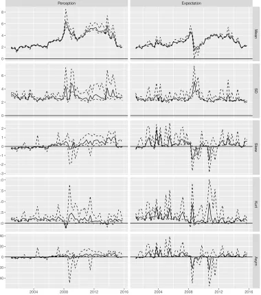
Figure 5 plots the posterior medians of the five moments of the distributions of inflation perceptions and expectations, respectively, during 2001Q1–2015Q4. We plot 68% error bands instead of 95% error bands, since the latter are often too wide to be informative for higher-order moments.
(Figure 5)
The estimated means of inflation perceptions and expectations seem reasonable and precise with narrow error bands. The means of inflation expectations are more stable than those of perceptions, staying around 2–4%, though not perfectly constant (anchored); hence individuals may expect that inflation fluctuations are temporary, though some per-sistence remains for one year.
The estimated standard deviations of inflation perceptions and expectations are some-times imprecise. This is perhaps because our interval data have little information about the dispersion of the underlying variable, especially when the majority of the respondents choose the last interval with an open end (“Up by 5% or more”). We still see that the standard deviations of inflation perceptions are often slightly larger than those of expec-tations; hence individuals may have private information when they perceive inflation, but expect its fluctuations to be temporary.
The estimated skewnesses of inflation perceptions and expectations seem reasonably precise, changing signs over time. The mean and skewness tend to move in the same direction, especially for inflation perceptions; hence responses to news on inflation are perhaps not uniform but heterogeneous among individuals.
The estimated kurtoses of inflation perceptions and expectations are often (but not always) imprecise. This is because our interval data have little information about the tails of the distribution of the underlying variable. We still see that the excess kurtoses are mostly positive for both inflation perceptions and expectations.
5.5 Estimation Including the Indifference Limen
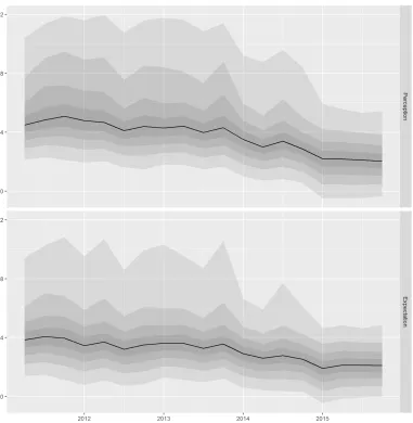
Next, we estimate the model with a common indifference limen among individuals. This may improve estimation efficiency, since we have two more intervals and use prior in-formation about the indifference limen (−∞ < γl < 0 < γu < 1). Figure 6 plots the posterior medians of the five moments and the indifference limens for inflation perceptions and expectations, respectively, during 2001Q1–2015Q4, together with 68% error bands.
(Figure 6)
We see that the estimated means and standard deviations are almost identical to the previous results with no indifference limen. Though we use more information in estimation, especially when many respondents choose categories 1–3, the differences in the 68% error bands are hardly visible. The estimated skewnesses, excess kurtoses, and asymmetries in the tails are sometimes slightly larger in magnitude than the previous results with no indifference limen. This is perhaps because with two more intervals, the data have more information about the tails of the underlying distribution.
The estimated indifference limens for inflation perceptions and expectations are both time-varying, and mostly asymmetric around 0. In particular, given our weakly informa-tive prior about the indifference limen, the lower bounds are often far below−1.0%. The upper bounds are around .0–.4% until early 2008, and .2–.6% since then. The error bands are wider for lower bounds than for upper bounds. This is perhaps because category 1 (“Gone/Go down”) has no lower bound and often has fewer observations than category 3 (“Up by 1% or less”).
5.6 Using Data with More Intervals
Finally, we estimate the model using data with 18 intervals including an indifference limen, which have been available since 2011Q2. With further questions to those who have chosen either category 1 or 8, the respondents now virtually choose from the following 18 intervals:
1. Down by 5% or more
2. Down by 4% but less than 5%
6. Down by 1% or less
7. Not changed/change
8. Up by 1% or less
. . .
17. Up by 9% but less than 10%
18. Up by 10% or more
Since −1 < γl < 0 < γu < 1, our weakly informative prior about the indifference limen now setsλ0 :=−1 andυ0:= 1. With 18 intervals, the NUTS works well without adjusting
the tuning parameters; thus we use the default values for all tuning parameters.
Figure 7 plots the posterior medians of the moments and indifference limens for in-flation perceptions and expectations, respectively, during 2011Q2–2015Q4. We also plot 95% error bands here instead of 68% error bands, since the former are narrow enough to be informative even for higher-order moments.
(Figure 7)
The estimated means are similar to the previous results using data with six or eight intervals during 2011Q2–2015Q4, except that the error bands are often narrower. The means are higher for inflation perceptions than for expectations when they are both high, but close to each other when they are 2–3%. Thus individuals may expect the inflation rate to fluctuate around 2–3% in the long run.
The estimated standard deviations are slightly larger than the previous results using data with six or eight intervals during 2011Q2–2015Q4, with much narrower error bands. This is perhaps because with 18 intervals, the data have much more information about the dispersion of the underlying distribution. The standard deviations for inflation perceptions and expectations are close to each other. The mean and standard deviation tend to move in the same direction. Thus individuals may agree with inflation perceptions and expectations when they are low, but not when they are high.
skewnesses are positive for both inflation perceptions and expectations, and slightly higher for expectations than for perceptions. The mean and skewness tend to move in the opposite directions.
The estimated kurtoses are also often larger than the previous results using data with six or eight intervals during 2011Q2–2015Q4. The excess kurtoses are mostly positive for both inflation perceptions and expectations, and higher for expectations than for percep-tions. The mean and kurtosis tend to move in the opposite direcpercep-tions.
The estimated asymmetries in the tails are often much larger than the previous results using data with six or eight intervals during 2011Q2–2015Q4. The asymmetries in the tails are positive for both inflation perceptions and expectations, and higher for expectations than for perceptions. The mean and asymmetry tend to move in the opposite directions. Overall, higher-order moments tend to move in the same directions. This may suggest existence of consistently positive outliers.
The estimated indifference limens, especially the lower bounds, differ from the previous results using data with eight intervals during 2011Q2–2015Q4. The upper bounds are around .3–.7% for perceptions and .4–.6% for expectations. Given the stronger prior information, the lower bounds stay above−1.0%. They are often below −.7%, however, and sometimes close to −1.0%. Thus the indifference limens are still often asymmetric around 0.
In addition to moments, quantiles help us to see the whole shape of a distribution. Figure 8 plots the posterior medians of the deciles of inflation perceptions and expectations during 2011Q2–2015Q4.13 These plots seem useful for monitoring the distributions of
inflation perceptions and expectations.
(Figure 8)
6
INFORMATION RIGIDITY IN THE UK
Information rigidity prevents one from forming full-information rational expectations. To measure and test for the degree of information rigidity, Coibion & Gorodnichenko (2015) give a simple framework that requires only the historical means of the distributions of
13
expectations. When only aggregate interval data are available, our method helps to obtain the mean of the possibly multi-modal underlying distribution. To illustrate such a use of our method, we measure the degrees of information rigidity in public inflation perceptions and expectations in the UK.
Consider individuals forming h-step ahead forecasts of a time series {yt}. A sticky information model proposed by Mankiw & Reis (2002) assumes that an individual receives no information with probabilityλ∈[0,1] at each date. Let ¯ye
t+h|t be the average forecast ofyt+h at date tamong individuals. Then for all t,
¯
ye
t+h|t:= (1−λ) Et(yt+h) +λ(1−λ) Et−1(yt+h) +λ2(1−λ) Et−2(yt+h) +· · · = (1−λ) Et(yt+h) +λ[(1−λ) Et−1(yt+h) +λ(1−λ) Et−2(yt+h) +· · ·]
= (1−λ) Et(yt+h) +λy¯et+h|t−1 (30)
or
Et(yt+h) = 1 1−λy¯
e t+h|t−
λ
1−λy¯
e t+h|t−1
= ¯yte+h|t+ λ 1−λ
(
¯
yet+h|t−y¯et+h|t−1) (31)
This gives a simple regression model with no intercept for the ex post forecast error
yt+h−y¯te+h|t given the ex ante mean forecast revision ¯yte+h|t−y¯te+h|t−1 such that for allt,
Et(yt+h−y¯te+h|t
)
=β(y¯te+h|t−y¯et+h|t−1) (32)
whereβ :=λ/(1−λ)≥0, or
yt+h−y¯et+h|t=β
(
¯
ye
t+h|t−y¯te+h|t−1 )
+ut+h|t (33)
whereut+h|t:=yt+h−Et(yt+h).14 One can estimateβ by OLS, from which one can recover
λ=β/(1 +β)∈[0,1).
One may observe only {y¯e t+h|t
}
instead of {y¯e
t+h|t,y¯et+h|t−1 }
. In such a case, one can
14
A noisy information model gives the same regression model if {yt}is AR(1); see Coibion &
consider an alternative model such that for allt,
yt+h−y¯te+h|t=β
(
¯
yte+h|t−y¯et+h−1|t−1)+vt+h|t (34)
where
vt+h|t:=ut+h|t−β
(
¯
yte+h|t−1−y¯te+h−1|t−1) (35)
This is not a regression model; hence one must apply the IV method instead of OLS, where the IV must be a white noise sequence. Coibion & Gorodnichenko (2015, p. 2663) use the change in the log oil price as the IV when measuring information rigidity in inflation expectations.
Let {Pt} be the quarterly series of the price level and πt := 100 ln(Pt/Pt−4) be the
annual inflation rate in per cent. Consider information rigidity inh-step ahead forecasts of
{πt}, whereh= 0 (nowcasts) for inflation perceptions andh= 4 for inflation expectations. We use the CPI and RPI for{Pt}, whose data are available at the website of the Office for National Statistics of the UK. The CPI and RPI inflation rates are somewhat different; see Figure 9.
(Figure 9)
Let ¯πe
t+h|t be the mean of the distribution of inflation perceptions (h = 0) or expec-tations (h = 4). Forh = 0,4, we apply our method to estimate ¯πe
t+h|t repeatedly during 2001Q1–2015Q4, assuming a normal distribution (K = 1) or a mixture of two normal distributions (K = 2) with or without an indifference limen.15 The resulting {π¯e
t+h|t
}
are somewhat different.
Since it is unclear if individuals forecast the CPI, RPI, or something else, to control for the possible bias in forecasts, we add an intercept to equation (34). We estimate the linear model by the IV method (2SLS). For IVs, in addition to a constant, we use the Brent Crude Oil Price in US dollars and the GBP/USD exchange rate, which are downloadable from Federal Reserve Economic Data (FRED). To make the IVs white noise sequences, we take the difference in log, and prewhiten each series by fitting a univariate AR(2) model
15
for the full sample period and extracting the residuals.16 We use gretl 2016d for these analyses.
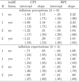
Table I summarizes the estimation results. We find the following:
1. The intercepts are negative for both the CPI and RPI and for both inflation percep-tions and expectapercep-tions, and significant except for expectapercep-tions relative to the RPI, suggesting forecast biases. The biases are larger for the CPI and perceptions than for the RPI and expectations.
2. The slopes are positive for both the CPI and RPI and for both inflation percep-tions and expectapercep-tions, though insignificant for the CPI. For the RPI, the size and significance of the slope depend on how we estimate the means of the distributions of inflation perceptions and expectations, i.e., the choice of the number of mixture components and whether we include the indifference limen or not.
3. If we believe that individuals forecast the RPI, assumeK = 2, and include the indif-ference limen when estimating the means of the distributions of inflation perceptions and expectations, then the slopes are insignificant, perhaps because of the short sam-ple length (59 for perceptions and 55 for expectations). Though insignificant, the implied λis .50 for β = 1.01 and .37 for β =.60; i.e., information rigidity is higher for perceptions than for expectations.17
(Table I)
To sum up, we find that evidences of information rigidity among UK individuals fore-casting inflation depend not only on what prices we assume they forecast, but also on how we model the distributions of their inflation perceptions and expectations. Thus we recommend fitting a flexible distribution, e.g., a mixture distribution, to aggregate interval data on inflation perceptions and expectations.
16
The full sample periods are 1987Q4–2015Q4 for the change in the log oil price and 1971Q2–2015Q4 for the change in the log exchange rate.
17
7
DISCUSSION
To estimate the distributions of public inflation perceptions and expectations in the UK, we study Bayesian analysis of a normal mixture model for interval data with an indifference limen. Since the boundaries of an indifference limen are similar to cutpoints in an ordered response model, the Gibbs sampler and M–H algorithm are slow to converge for large samples. We find that the NUTS converges fast even for large samples. Thus the NUTS is useful especially when one must apply MCMC repeatedly, which is our case.
One can extend and improve our method in several ways. Here we list some directions for future work:
1. Instead of assuming a common indifference limen among individuals (or simply ig-noring it), one can model heterogeneous indifference limens, say, assuming beta dis-tributions for the boundaries. This makes the likelihood function more complicated, but seems worth trying.
2. One can estimate the number of mixture components instead of fixing it a priori. Common model selection criteria may be inappropriate for finite mixture models, however; see Gelman et al. (2014, p. 536). Since HMC does not allow discrete parameters, MCMC for the number of components requires combining HMC with another MCMC method. A model with a few components is a special case of a model with many components; thus one may simply consider the latter with a suitable prior on the number of components; see Gelman et al. (2014, p. 536).
3. Instead of fitting a distribution each quarter separately, one can use multiple samples jointly to study the dynamics of the underlying distribution directly. For time series analysis of repeated interval data, one may need a state-space model with a nonlinear measurement equation.
Micro data from the Bank of England/GfK NOP Inflation Attitudes Survey are now publicly available at the website of the Bank of England. This suggests the following extensions of this paper:
2. One can study the determinants of individual inflation perceptions and expecta-tions, separately or jointly, by interval regression or its extension that allows for an indifference limen. This is an extension of Blanchflower & MacCoille (2009).
Thus the micro data will greatly help us to study the formation, dynamics, and interaction of inflation perceptions and expectations.
References
Albert, J. H., & Chib, S. (1993). Bayesian analysis of binary and polychotomous response data. Journal of the American Statistical Association, 88, 669–679. doi: 10.2307/2290350
Alston, C. L., & Mengersen, K. L. (2010). Allowing for the effect of data binning in a Bayesian normal mixture model. Computational Statistics & Data Analysis, 54, 916– 923. doi: 10.1016/j.csda.2009.10.003
Armantier, O., Bruine de Bruin, W., Potter, S., Topa, G., van der Klaauw, W., & Zafar, B. (2013). Measuring inflation expectations. Annual Review of Economics,5, 273–301. doi: 10.1146/annurev-economics-081512-141510
Betancourt, M., & Girolami, M. (2015). Hamiltonian Monte Carlo for hierarchical models. In S. K. Upadhyay, U. Singh, D. K. Dey, & A. Loganathan (Eds.), Current trends in bayesian methodology with applications (pp. 79–102). CRC Press.
Biernacki, C. (2007). Degeneracy in the maximum likelihood estimation of univariate Gaussian mixtures for grouped data and behavior of the EM algorithm. Scandinavian Journal of Statistics,34, 569–586. doi: 10.1111/j.1467-9469.2006.00553.x
Binder, C. C. (2015). Measuring uncertainty based on rounding: New method and appli-cation to inflation expectations. (Available at SSRN) doi: 10.2139/ssrn.2576439
Chen, M.-H., & Dey, D. K. (2000). Bayesian analysis for correlated ordinal data models. In D. K. Dey, S. K. Ghosh, & B. K. Mallick (Eds.),Generalized linear models: A Bayesian perspective (pp. 133–157). Marcel Dekker.
Chib, S., & Greenberg, E. (1995). Understanding the Metropolis–Hastings algorithm.
American Statistician,4, 327–335. doi: 10.1080/00031305.1995.10476177
Coibion, O., & Gorodnichenko, Y. (2015). Information rigidity and the expectations formation process: A simple framework and new facts. American Economic Review,
105, 2644–2678. doi: 10.1257/aer.20110306
Cowles, M. K. (1996). Accelerating Monte Carlo Markov chain convergence for cumulative-link generalized linear models. Statistics and Computing,6, 101–111. doi: 10.1007/BF00162520
Fr¨uhwirth-Schnatter, S. (2006). Finite mixture and markov switching models. Springer.
Gelman, A., Carlin, J. B., Stern, H. S., Dunson, D. B., Vehtari, A., & Rubin, D. B. (2014).
Bayesian data analysis (3rd ed.). CRC Press.
Geweke, J. (2007). Interpretation and inference in mixture models: Simple MCMC works. Computational Statistics & Data Analysis, 51, 3529–3550. doi: 10.1016/j.csda.2006.11.026
Hoffman, M. D., & Gelman, A. (2014). The No-U-Turn Sampler: Adaptively setting path lengths in Hamiltonian Monte Carlo. Journal of Machine Learning Research,15, 1593–1623.
Kamada, K., Nakajima, J., & Nishiguchi, S. (2015). Are household inflation expectations anchored in Japan? (Working Paper No. 15-E-8). Bank of Japan.
Kiefer, J., & Wolfowitz, J. (1956). Consistency of the maximum likelihood estimator in the presence of infinitely many incidental parameters. Annals of Mathematical Statistics,
Lahiri, K., & Zhao, Y. (2015). Quantifying survey expectations: A critical review and generalization of the Carlson–Parkin method. International Journal of Forecasting,31, 51–62. doi: 10.1016/j.ijforecast.2014.06.003
Liu, J. S., & Sabatti, C. (2000). Generalized Gibbs sampler and multigrid Monte Carlo for Bayesian computation. Biometrika,87, 353–369. doi: 10.1093/biomet/87.2.353
Lombardelli, C., & Saleheen, J. (2003). Public expectations of UK inflation. Bank of England Quarterly Bulletin,43, 281–290.
Mankiw, N. G., & Reis, R. (2002). Sticky information versus sticky prices: A proposal to replace the new Keynesian Phillips curve. Quarterly Journal of Economics, 117, 1295–1328. doi: 10.1162/003355302320935034
Mankiw, N. G., Reis, R., & Wolfers, J. (2004). Disagreement about inflation expectations. In M. Gertler & K. Rogoff (Eds.), NBER macroeconomics annual 2003 (Vol. 18, pp. 209–248). MIT Press.
Manski, C. F. (2004). Measuring expectations. Econometrica, 72, 1329–1376. doi: 10.1111/j.1468-0262.2004.00537.x
Manski, C. F., & Molinari, F. (2010). Rounding probabilistic expectations in surveys.
Journal of Business & Economic Statistics,28, 219–231. doi: 10.1198/jbes.2009.08098
Murasawa, Y. (2013). Measuring inflation expectations using interval-coded data.
Oxford Bulletin of Economics and Statistics, 75, 602–623. doi: 10.1111/j.1468-0084.2012.00704.x
Nandram, B., & Chen, M.-H. (1996). Reparameterizing the generalized linear model to ac-celerate Gibbs sampler convergence.Journal of Statistical Computation and Simulation,
54, 129–144. doi: 10.1080/00949659608811724
Nardo, M. (2003). The quantification of qualitative survey data: A critical assessment.
Neal, R. M. (2011). MCMC using Hamiltonian dynamics. In S. Brooks, A. Gelman, G. L. Jones, & X.-L. Meng (Eds.), Handbook of Marcov chain Monte Carlo (pp. 113– 162). Chapman & Hall/CRC.
Papaspiliopoulos, O., Roberts, G. O., & Sk¨old, M. (2003). Non-centered parameterisations for hierarchical models and data augmentation. In J. M. Bernardo et al. (Eds.),Bayesian statistics 7 (pp. 307–326). Oxford University Press.
Papaspiliopoulos, O., Roberts, G. O., & Sk¨old, M. (2007). A general framework for the parametrization of hierarchical models. Statistical Science, 22, 59–73. doi: 10.1214/088342307000000014
Pesaran, M. H., & Weale, M. (2006). Survey expectations. In G. Elliot, C. W. J. Granger, & A. Timmermann (Eds.), Handbook of economic forecasting (Vol. 1, pp. 715–776). Amsterdam: Elsevier.
R Core Team. (2016). R: A language and environment for statistical computing [Computer software manual]. Vienna, Austria. Retrieved fromhttps://www.R-project.org
Richardson, S., & Green, P. J. (1997). On Bayesian analysis of mixtures with an unknown number of components (with discussion).Journal of the Royal Statistical Society: Series B (Statistical Methodology),59, 731–792. doi: 10.1111/1467-9868.00095
Sinclair, P. (Ed.). (2010). Inflation expectations. Routledge.
Stan Development Team. (2016). RStan: the R interface to Stan. Retrieved from
http://mc-stan.org/ (R package version 2.14.1)
Terai, A. (2010). Estimating the distribution of inflation expectations.Economics Bulletin,
2001Q1 2008Q3
down nochange up0−1 up1−2 up2−3 up3−4 up4−5 up5− down nochange up0−1 up1−2 up2−3 up3−4 up4−5 up5− 0
[image:29.595.107.491.94.284.2]250 500 750 1000
Figure 1: Distributions of inflation perceptions in the UK (2001Q1 and 2008Q3)
2011Q2
2015Q4
d5− d4−5 d3−4 d2−3 d1−2 d0−1 0 u0−1 u1−2 u2−3 u3−4 u4−5 u5−6 u6−7 u7−8 u8−9 u9−10 u10− 0
100 200 300
0 100 200 300
[image:29.595.107.488.334.722.2]0 1000 2000 3000 4000
2004 2008 2012 2016
Perception Expectation
[image:30.595.104.492.272.531.2]P
erception
Expectation
2004 2008 2012 2016
0.00 0.25 0.50 0.75 1.00
0.00 0.25 0.50 0.75 1.00
[image:31.595.104.485.207.596.2]up5− up4−5 up3−4 up2−3 up1−2 up0−1 nochange down
Perception Expectation
Mean
SD
Sk
e
w
K
ur
t
Asym
2004 2008 2012 2016 2004 2008 2012 2016
0 2 4 6 8
0 2 4 6
−3 −2 −1 0 1 2
0.0 2.5 5.0 7.5 10.0
[image:32.595.112.492.182.611.2]−40 −20 0 20 40
Perception Expectation
Mean
SD
Sk
e
w
K
ur
t
Asym
Gam_u
Gam_l
2004 2008 2012 2016 2004 2008 2012 2016
0 2 4 6 8
0.0 2.5 5.0 7.5
−4 −2 0 2
0 5 10 15 20
−150 −100 −50 0
0.0 0.2 0.4 0.6
[image:33.595.111.492.90.699.2]−10 −5 0
Perception Expectation Mean SD Sk e w K ur t Asym Gam_u Gam_l
2012 2013 2014 2015 2012 2013 2014 2015
[image:34.595.113.490.91.697.2]0 2 4 6 0 1 2 3 4 0 1 2 3 0 5 10 15 0 40 80 120 0.0 0.2 0.4 0.6 0.8 −1.00 −0.75 −0.50 −0.25 0.00
Figure 8: Posterior medians of the deciles of the distributions of inflation perceptions and expectations in the UK during 2011Q2–2015Q4.
0 2 4
2004 2008 2012 2016
cpi rpi
[image:35.595.106.492.535.727.2]Table I: 2SLS regressions of the ex post forecast errors on the ex ante mean forecast revisions
indiff. CPI RPI
K limen intercept slope intercept slope inflation perceptions (h= 0)
1 no −1.10 1.17 −.45 2.32 (.12) (.71) (.24) (.96) 1 yes −1.09 1.18 −.45 2.33
(.12) (.71) (.24) (.96) 2 no −1.22 .31 −.58 1.04
(.17) (.50) (.29) (.66) 2 yes −1.21 .29 −.57 1.01
(.16) (.54) (.28) (.65) inflation expectations (h= 4)
1 no −.71 .85 −.04 1.68 (.24) (.85) (.35) (.82) 1 yes −.71 .85 −.04 1.68
(.24) (.85) (.35) (.82) 2 no −.72 .25 −.05 .93
(.26) (.76) (.35) (.78) 2 yes −.69 .07 −.01 .60
(.27) (.69) (.35) (.69)