Munich Personal RePEc Archive
Amazon Mechanical Turk Workers Can
Provide Consistent and Economically
Meaningful Data
Johnson, David and Ryan, John
University of Central Missouri
12 July 2018
Online at
https://mpra.ub.uni-muenchen.de/88450/
Amazon Mechanical Turk Workers Can Provide
Consistent and Economically Meaningful Data
David Johnson
∗University of Central Missouri
John Barry Ryan
†Stony Brook University
July 12, 2018
Abstract
We explore the consistency of the characteristics of individuals who participate in studies posted on Amazon Mechanical Turk (AMT). The primary individuals analyzed in this study are subjects who participated in at least two of eleven experiments that were run on AMT between September of 2012 to January of 2018. We demonstrate subjects consistently report a series of demographic and personality characteristics. Further, subjective willingness to take risk is found to be significantly correlated with decisions made in a simple lottery experiment with real stakes - even when the subjec-tive risk measure is reported months, sometimes years, in the past. This suggests the quality of data obtained via AMT is not significantly harmed by the lack of control over the conditions under which the responses are recorded.
∗Department of Economics and Finance, University of Central Missouri, Warrensburg,
MO 64093, U.S.A. Telephone: 1-336-639-2190. Email: [email protected]
†Department of Political Science, Stony Brook University, Stony Brook, NY 11794, U.S.A.
1 Introduction
Amazon Mechanical Turk (also known as AMT or MTurk) has become an increasingly
com-mon tool for researchers in social sciences (e.g.,Clifford,2014;Verkoeijen and Bouwmeester,
2014; Milita et al.,2017). This is partly because researchers are looking for experimental
samples that are more heterogeneous than student samples and cheaper than samples
re-cruited by survey firms. However, critics of AMT worry that the results of studies using AMT
are unreliable and not economically meaningful. The reasoning behind such worries are
often based off of some mixture of formal criticisms (e.g., frequency of participation and
unrepresentative samples) that are discussed in the academic literature (c.f., Krupnikov
and Levine, 2014; Huff and Tingley, 2015), and informal criticisms that crop up in
ref-eree reports (e.g., loss of experimental control, low incentives, and overall subject quality).
Given that experiments performed on AMT generally replicate the results from studies on
nationally representative samples (Mullinix et al.,2015) and laboratory studies (Horton et
al.,2011), these criticisms – particularly, the informal flavor – seem puzzling.
Naturally the observation of poor quality responses could be the result of rational
de-cision making on the part of the respondent. For example, it is easy to imagine that some
respondents may (or may not) have beliefs/preferences that align with a study’s goals. If
the study’s goals are deciphered by the respondent, the respondent could answer questions
in a manner to achieve or undermine the study’s goals rather than responding honestly.
Additionally, because respondents are paid for each survey they complete, there is the
in-centive to complete surveys as quickly as possible. For instance, if a respondent has 10
minutes to complete an online survey and mindlessly completes the 10 minute survey in 5
minutes, they are free to complete another survey and will get paid for both. Hence,
regard-less of whether respondents are carefully reading the questions or careregard-lessly responding,
they might give poor quality responses.
platform by demonstrating that AMT worker responses are consistent across time and
cor-related, in the expected direction, with decisions that are made when there are real stakes
present. Our data is from eleven different experiments run on AMT from September of 2012
to January of 2018. In each of these experiments, we collected at least two of the following
measures: age, gender, impulsivity, and subjective willingness to take risk. We take
advan-tage of the fact that AMT data sets report workers’ anonymous “worker id” numbers and use
this information to track worker responses over time. We show differences in responses are
small – which would be consistent with measurement error – both to single questions and
a multi-item index.1 Further, we demonstrate that self-reported risk measures are highly
correlated with a financially incentivized measure of risk. This is important because it
sug-gests the consistency is economically meaningful and not the result of some decision rule
used to complete surveys more quickly – for example, always picking the first option.
Be-cause we can predict the respondent’s incentivized behavior with self-reported measures
taken at the same time or months or, in some cases, even years before, this suggests AMT
respondents provide valid measures of variables that are important to social scientists.
2 AMT and Inconsistent Responses
AMT is an online labor market made up of workers (respondents/subjects) and requestors
(researchers). Requestors on AMT post human intelligence tasks (HITs) that are then
com-pleted by workers in exchange for payment. In the social sciences, these HITs are often
experiments (e.g., Clifford and Gaskins, 2016; Del Ponte et al.,2017; Milita et al., 2017)
and are seen as an alternative to laboratory experiments that use student samples
(Good-man et al.,2013). Each HIT on AMT pays workers a fixed participation fee for completing
a HIT. These fixed participation fees are typically quite small and range from $0.05 to
1In fact, the responses to the question about risk preference are more reliable than
$1.00. This participation fee is analogous to the show-up payments paid to subjects in
laboratory economics experiments. Requestors also have the option of paying workers a
bonus. A convenient feature of these bonuses is that they are individually assigned after
the requestor has observed workers’ responses. This means requestors can observe
work-ers’ behaviors/decisions and pay them based off of their observed behavior/decisions. Like
the participation fees, these bonuses are quite small relative to laboratory payments.
Demographically, AMT workers are significantly more varied than university subject
pools (Ipeirotis, 2010; Buhrmester et al.,2011; Behrend et al., 2011). For example, it is
common to observe workers who report to be as young as 18 and as old as 65. However,
American workers are still younger and more ideologically liberal than the overall U.S.
population (Berinsky et al.,2012). More importantly, for the purposes of this paper and
others using AMT, American workers on AMT generally have a lower reported income (c.f.,
Paolacci et al.,2010;Berinsky et al.,2012;Levay et al.,2016) are more likely to report to
be unemployed (e.g.,Ipeirotis,2010;Goodman et al.,2016).
This suggests that the money earned from completing HITs might be especially
valu-able to AMT workers. Since the HITs generally pay small amounts, the only way to earn
even minimum wage is to complete many HITs. However, this could lead to poor
re-sponses as respondents engage in satisficing or some quick decision rule (for example,
always choose the middle category). It could also lead to response instability, one of the
most common issues in social science surveys (Converse, n.d.). Zaller(1992) notes that
one way to cure response instability is to encourage respondents to “stop and think” prior
to answering. For these AMT respondents, stopping to think is costly as time spent thinking
is time not spent earning money for completing another HIT.
At the same time, survey experiments conducted on the platform have been shown to
replicate the results from surveys on representative samples (Berinsky et al.,2012;Mullinix
Ex-perimental effects would potentially replicate if responses in both samples were of poor
quality. AMT workers have a financial incentive to finish quickly, but respondents to a
more traditional survey also would want to finish quickly.
As part of an effort to improve the quality of responses, experimental economists
ask respondents to participate in tasks with real stakes in order to measure underlying
attitudes. For example, one could measure intergroup affect with survey questions, but
measuring affect via a trust or dictator games avoids issues of social desirability (Fowler
and Kam, 2007; Carlin and Love, 2013). By offering real stakes to answer a question,
researchers can incentivize careful responding. An AMT worker, who answers the real
stakes question too quickly, risks lower earnings which may defeat the purpose of quick
responding. However, one could argue that the cost of this behavior is mitigated by the
relatively low stakes. Hence, to demonstrate that AMT workers provide quality data, we
need to demonstrate both that the responses are consistent across time, but also that the
measures obtained via survey questions are consistent with those from a real (but low)
stakes task.
3 Data
We ask two central questions: 1) is the data provided by AMT workers consistent? and 2)
if so, are workers’ responses economically meaningful – i.e., do their responses to survey
questions correlate with their performance in a real stakes task? The data we use is from
eleven different experiments which were run from 2012 to 2018. To avoid selection bias,
we use data from all of the experiments author one has run on AMT that asked workers
to report at least two of the measures above and have access to their worker identification
number (workerid) and the date the experiment was posted.2 The dates of the experiments
2A description of each experiment is found in Appendix section 5. All experimental data
and the number of observations in each experiment are found in Table E.1 in the Appendix.
The timing of each of the variables of interest (e.g., age and impulsiveness test) varies
widely across experiments. For example, in some experiments workers were asked about
their willingness to take risk prior to the experiment (to conceal a treatment assignment
variable) and, in others, the question occurred after the main experiment.
3.1 Questions
In assessing the consistency of workers’ responses we evaluate four variables. The first
two are basic demographic variables: age and gender. These measures provide only a
low-bar test as answering those questions quickly and carelessly would take about as long as
answering the questions accurately. It will serve to demonstrate that AMT workers are not
“trolling” researchers (Lopez and Hillygus,2018).
We perform more comprehensive analyses of two respondent personality traits:
im-pulsiveness and willingness to take risk. Imim-pulsiveness is a commonly studied trait in the
psychology of criminals (Farrington,1998) and has been used in political science to explain
differences between liberals and conservatives (McAdams et al., 2013), partisan strength
(Hatemi et al.,2009) and political violence (McDermott et al.,2013). Impulsiveness is
mea-sured using the Barratt Impulsivity Test (Stanford et al.,2009). Respondents indicate how
often they engage in thirty different activities (e.g., “I plan tasks carefully”) using a four
point scale ranging from “Rarely/Never" (1) to “Almost Always/Always" (4). A worker’s
impulsiveness score is the sum of their responses.3 To demonstrate that workers
consis-tently report their level of impulsiveness, we use both workers’ responses to each of the
impulsiveness questions as well as their total score on the instrument.
Willingness to take risk is measured using the general risk attitudes question from
the German Socio-Economic Panel Survey (SOEP) which was popularized inDohmen et al.
(2011). The English translation of the question is as follows:
How do you see yourself: Are you generally a person who is fully prepared to take risks or do you try to avoid taking risks?
Workers answer this question on an 11 point scale ranging from 0 to 10 - with 0
corresponding to “I avoid risk" and 10 corresponding to “Fully prepared to take risks.”
Additionally, in two of the experiments respondents were asked to choose to play one
lottery from a list of several lotteries; this is a common way to measure an individual’s risk
profile in experimental economics (e.g.,Holt and Laury,2002; Dave et al.,2010). We will
explain the details of the real stakes task later when we examine how it correlates with the
answer to the SOEP risk attitudes question.
A convenient feature of the data sets generated using AMT is that they not only
in-clude workers’ decisions and responses but also a unique randomly generated worker
iden-tification number (workerid) and the date at which the HIT was posted online. We use the
workerid to link the responses of workers who participated in at least two of the
experi-ments presented in Table E.1 in the Appendix. The date is used to establish the order of the
responses – allowing us to compare a respondent’s first response to their future responses.
3.2 AMT Workers
In the eleven experiments, there are 5,347 observations. 3,566 workers completed a single
experiment. 730 workers completed at least two, and 223 workers completed three or
more experiments. The average number of experiments completed by workers is 1.24 and
the most experiments completed by a worker is eight. We did not contact workers who
participated in one study to participate in future studies. Hence, the fact that respondents
appear in this study in a panel nature is purely by chance. 4,127 workers reported their
completed the Barratt Impulsivity Test.4
Table1presents the summary statistics of the workers who participated in the
exper-iments.5 Each variable in Table 1 contains subscripts indicating a group and a response
time. The first subscript corresponds to the order of the workers’ response (i.e., 1 if first; 2
if last). Workers are classified into one of two groups. The first group (group 1) are workers
who participated in one experiment. The second group (group 2) are workers who
partic-ipated in two or more experiments. The group is indicated by the second subscript (i.e., 1
if group 1; 2 if group 2). For example, Risk1,2 is the average earliest reported willingness
to take risk for workers who completed more than one experiment.
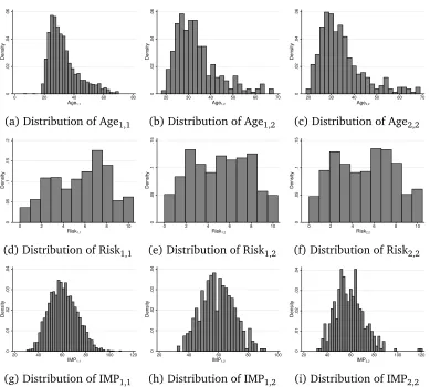
The distributions of Age, Risk, and IMP by group, and order of response are found
in Figure 4. Figure 4 and Table 1 suggest that there are differences in the workers who
completed more than one experiment compared to those who only completed a single
ex-periment. Workers who completed more than one experiment are significantly more likely
to report being male (test of proportions: 0.561 vs 0.628, p = 0.001), are less
impul-sive (t-test: 60.623 vs 58.329, p < 0.001; u-test: p < 0.001), are less willing to take
risk (t-test: 5.364 vs 5.037, p = 0.005; u-test: p = 0.005), and older (t-test: 32.149 vs
33.856, p<0.001; u-test: p<0.001) than workers who completed a single experiment.6
This means the experienced AMT participants have somewhat different characteristics than
those who are less experienced, which may lead to questions regarding external validity
relating to the consistency of responses. Yet, it does not affect our ability to test whether
4A breakdown of average responses by the day of the week the batch of the HIT is posted
is found in section 1 of the Appendix. Detailed analysis of “day of the week” effects are not the primary purpose of this paper but is available upon request.
5Careful readers will note that the sum of the variables in Table1do not add up to the
“correct” total. This is due to the fact that workers could have completed experiments that did not ask them to report one or two of the measures. So, for example, while a worker could have completed more than one experiment, she could have actually only reported her age once.
Table 1: Summary Statistics
Responded Once
Variable Obs Mean Std. Min Max
Male1,1 3398 0.561 0.496 0 1
Age1,1 2136 32.149 10.028 6 69
Risk1,1 3090 5.364 2.691 0 10
IMP1,1 2055 60.623 11.628 30 110
Responded More than Once (First Response)
Variable Obs Mean Std. Min Max
Male1,2 678 0.645 0.479 0 1
Age1,2 418 33.117 9.536 18 67
Risk1,2 553 4.911 2.793 0 10
IMP1,2 406 58.628 11.106 32 92
Responded More than Once (Last Response)
Variable Obs Mean Std. Min Max
Male2,2 678 0.639 0.481 0 1
Age2,2 418 33.969 9.663 19 69
Risk2,2 553 4.929 2.824 0 10
IMP2,2 406 58.369 12.441 31 120
experienced and inexperienced workers provide economically meaningful responses.7
In the coming analysis, we will primarily consider the respondents who participated
in more than one study as those are the only respondents who we can show are consistent
in their responses. However, we will later use some participants who participated only once
to compare their responses to the risk question to their decisions made in the real stakes
lottery task. As we will demonstrate, the relationship between subjective risk preferences
and choices made in the incentivized lottery experiment, for workers who participated in
only one experiment, is not qualitatively different than the relationship observed in workers
who participated in more than one experiment.
4 Results
4.1 Age and Gender Consistency
As a “low-bar” test of the consistency of responses, we start by exploring workers’ first
reported gender and age and compare these responses to their final responses. The
av-erage number of days between first reported gender(age) and last reported gender(age)
is 401(289) days. Overall, 666 workers consistently reported their gender. 237 of these
workers reported being female and 429 of these workers reported being male. Eight(four)
workers first reported being male(female) but reported being female(male) in the last
ex-periment they completed. Thus, workers consistently report their gender 98.23 % of the
time.8
7Note that the averages presented in Table1do not match the averages and proportions
reported when we are comparing responses across groups. This is not a mistake but reflects
the fact not all HITs asked the same questions. See Footnote5for a more concrete example.
8Given that recent studies estimate that between 0.4% and 0.6% of the US population
identifies as transgender (Flores et al.,2016), some of the observed inconsistency possibly
re-Figure 1: Distribution of workers’ characteristics by group and completion order. 0 .02 .04 .06 Density
0 20 40 60 80
Age1,1
(a) Distribution of Age1,1
0
.02
.04
.06
Density
20 30 40 50 60 70
Age1,2
(b) Distribution of Age1,2
0
.02
.04
.06
Density
20 30 40 50 60 70
Age2,2
(c) Distribution of Age2,2
0 .05 .1 .15 .2 Density
0 2 4 6 8 10
Risk1,1
(d) Distribution of Risk1,1
0
.05
.1
.15
Density
0 2 4 6 8 10
Risk1,2
(e) Distribution of Risk1,2
0
.05
.1
.15
Density
0 2 4 6 8 10
Risk2,2
(f) Distribution of Risk2,2
0 .01 .02 .03 .04 Density
20 40 60 80 100 120
IMP1,1
(g) Distribution of IMP1,1
0 .01 .02 .03 .04 Density
20 40 60 80 100
IMP1,2
(h) Distribution of IMP1,2
0 .01 .02 .03 .04 Density
20 40 60 80 100 120
IMP2,2
(i) Distribution of IMP2,2
[image:12.612.105.494.168.518.2]418 workers reported their age more than once. The correlation between first and last
reported age is positive and significant (r=0.977,p<0.0001). The average reported age
when workers completed their first(last) experiment 33.12(33.97) which translates into
a difference of .85 years. While this difference is statistically significantly different from
zero (t-test: p<0.001) it is expected considering workers will age over the time between
experiments. Yet, this difference is not statistically different from the difference in the time
they last reported their age and first reported their age divided by 365 (t-test: 0.85 vs .793,
p = 0.174). Just as with gender there is some inconsistency. There are eight “Benjamin
Buttons” who got younger and five workers who aged more than was possible.9 Overall,
these results suggest, for simple demographic questions at least, MTurk respondents are
fairly consistent.
4.2 Consistency in Impulsivity
We now present results suggesting that workers are consistently reporting their impulsivity.
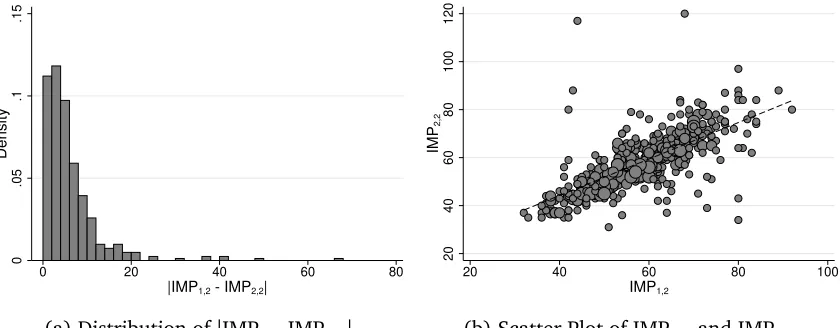
The distribution of the absolute difference between workers’ first and last Impulsiveness
Test score is found in Figure 2a. In Figure 2b, we present a scatter plot of IMP1,2 and
IMP2,2. The average time difference between workers’ first and last Impulsivity Test is 339
days. As with the previous demographics and characteristics, workers consistently report
their impulsivity.
The difference in workers’ first and last Impulsivity Test score is not statistically
dif-ferent (paired t-test: 58.628 vs 58.369, p = 0.5843). While the two scores are highly
correlated (r = 0.679, p < 0.001) the observed correlation is not as high as what is
re-ported being male and then subsequently rere-ported being female in two later experiments. Obviously, it is impossible to say whether or not the first response given by this worker was a mistake or not but it is noteworthy to mention that this worker was very consistent in their
reported willingness to take risk (Risk1,2=4 and Risk2,2=5) and impulsiveness (IMP1,2=52
and IMP2,2=49).
Figure 2: Distribution of the Absolute Differences and Scatter Plots of First and Last Impul-sivity Test Responses.
0
.05
.1
.15
Density
0 20 40 60 80
|IMP1,2 - IMP2,2|
(a) Distribution of|IMP1,2-IMP2,2|
20
40
60
80
100
120
IMP
2,2
20 40 60 80 100
IMP1,2
(b) Scatter Plot of IMP1,2and IMP2,2
Figure 2a presents the distribution of the absolute difference of workers’ first Impulsiveness Test score and final Impulsiveness Test score. Figure2bpresents a scatter plot of workers’ first Impulsiveness Test score (IMP1,2) and final reported willingness to take risk (IMP2,2). X-axis corresponds to first reported willingness to take risk/test score while y-axis is final reported willingness to take risk/test score. Dashed lines are fitted regression lines. Dot sizes, in the scatter plots, indicate the proportion of responses.
ported in Stanford et al. (2009) who finds a one month correlation across test scores of
0.83. As can be seen in Figure2a, this difference is being driven by a few very inconsistent
workers. For example, if we remove the eight most inconsistent workers (or less than 2 %
of the sample of workers who completed the Impulsivity Test more than once),r increases
to .804.10
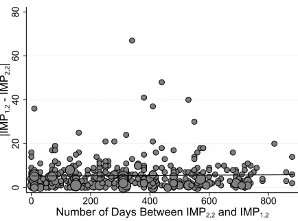
The number of days between measures does not affect the consistency of the
re-sponses. This can be seen in Figure 3 which plots the absolute difference between first
and last scores on the impulsivity measure on the y-axis and the number of days between
responses on the x-axis. When we estimate an OLS model using the absolute difference
as a dependent variable and the number of days between responses as the independent
10Interestingly, one of these workers inconsistently reported their gender which might
Figure 3: Difference in Impulsivity Test Responses Over Time.
0
20
40
60
80
|IMP
1,
2
-
IMP
2,
2
|
0 200 400 600 800
Number of Days Between IMP2,2 and IMP1,2
The solid lines is the fitted regression line. Dot sizes indicate the proportion of responses.
variable, we find the coefficient on the number of days between measures is small and not
statistically significant (coef=0.001,p=0.594,n=406).
In Appendix section 4, we present the result for each of thirty items in test. The
difference between initial and final responses to one item has a p-value less than 0.05 with
another two items having p-values less than 0.1. Given the multiple tests, we should adjust
our p-values for multiple comparisons. Whether we account for “false discovery rate” – the
expected proportion of false positives (Type I errors) (Benjamini and Hochberg,1995) – or
“Family-Wise Error Rate” – the probability of incorrectly rejecting even one null hypothesis
– using the common Bonferroni correction, there are no statistically significant differences
between the first and final responses to any of the items.
4.3 Consistency in Willingness to Take Risk
The distribution of the absolute difference between workers’ first and last reported
willing-ness to take risk is found in Figure4a. In Figure4b, we present a scatter plot of Risk1,2and
Risk2,2. The average time difference between workers’ first and last response to the risk
Figure 4: Distribution of the Absolute Differences and Scatter Plots of First and Last Impul-sivity Test Responses.
0
.1
.2
.3
.4
Density
0 2 4 6 8 10
|Risk1,2 - Risk2,2|
(a) Distribution of|Risk1,2-Risk2,2|
0
2
4
6
8
10
Risk
2,2
0 2 4 6 8 10
Risk1,2
(b) Scatter Plot of Risk1,2and Risk2,2
Figure4apresents the distribution of the absolute difference of workers’ first reported general willingness to take risk and final reported general willingness to take risk. Figure4b presents a scatter plot of workers’ first reported willingness to take risk (Risk1,2) and final reported willingness to take risk (Risk2,2). Dashed lines are fitted regression lines. Dot sizes, in the scatter plots, indicate the proportion of responses.
last time they completed an experiment is not statistically significant (paired t-test: 4.911
vs 4.929, p = 0.852) and, as expected, the responses themselves are highly correlated
(r =0.672, p<0.001). Further, the reported reliability (i.e., test and re-test correlation)
is higher than the 30-49 day reliability (r=0.60) reported in the SOEP manual (Richter et
al.,2017).
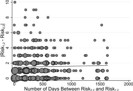
Additionally, we once again see no evidence that the difference in reported willingness
to take risk increases in the number of days between the first and last time it is reported. We
show this in Figure5which plots the absolute difference between first and last responses
to risk question on the y-axis and the number of days between responses on the x-axis.
When estimating the absolute difference between first and last response, with OLS, using
the number of days between responses as the independent variable, we find the coefficient
on the number of days between measures to be small and not statistically significant (coef=
Figure 5: Difference in Willing to Take Risk Over Time.
0
2
4
6
8
10
|Risk
1,
2
-
Risk
2,
2
|
0 500 1000 1500 2000
Number of Days Between Risk2,2 and Risk1,2
The solid lines is the fitted regression line. Dot sizes indicate the proportion of responses.
4.3.1 Risk Measured with Real Stakes
We have shown that AMT respondents provide consistent responses, but this does not
nec-essarily mean the data is of high quality or economically meaningful. Consistent responses
could be the result of careful consideration or a basic decision rule – for example, always
answer the middle option. We now show that the data AMT workers provide is
econom-ically meaningful. We do so by showing that subjective risk preferences correlate in the
expected direction with workers’ decisions in a simple real stakes task: an incentivized
lottery experiment (Johnson and Webb,2016;Gibson and Johnson,2018).11
In the experiment, workers are given a set of 20 lotteries (shown in Table 2) that
vary in the probability they will be successful and the payoff that will be paid if the lottery
turns out to be successful. Lotteries that are riskier (i.e., lower in index number) have a
higher payoff (if successful) while lotteries that are safer (i.e., higher in index number)
11Note here we are focusing on the control treatment ofJohnson and Webb(2016) that
had workers select a single lottery rather than a bundle of lotteries. Gibson and Johnson
have a lower payoff (if successful).12 After being shown the possible lotteries that they
can select, and each lottery’s expected value, workers are asked to select the lottery that
they wish to play for real stakes. The advantage of this simple risk task compared to some
others available is that the measure does not conflate risk preference and math ability as
is the case with some more complex measures, which makes it particularly suitable for the
environment and population.
The stakes of the experiment are quite low relative to laboratory experiments.
Work-ers, on average, earned about $1.15 for their decisions. 122 workers completed the lottery
experiment. The average subjective willingness to take risk of workers, taken at the time of
the incentivized experiment is 4.76. The correlation between these two variables is -0.332
and is statistically significant (p = 0.0002). The average index number of the lottery
se-lected by these workers is 11.75 which is statistically significantly greater than the index
number of the safer of two lotteries that are expected utility maximizing (lottery 11 in Table
2) assuming risk neutral preferences (t-test: p=0.039). Overall, roughly 67% of subjects
selected a lottery that is consistent with some degree of risk averse preferences. Of subjects
who completed the lottery experiment and a prior experiment in which they were asked to
report their general willingness to take risk, this figure rises to approximately 76%.
In bothJohnson and Webb(2016) and Gibson and Johnson(2018) workers also
re-ported their general willingness to take risk. 122 workers participated in either the control
treatment ofJohnson and Webb(2016) (n=47) orGibson and Johnson(2018) (n=75).
We now demonstrate that workers’ subjective willingness to take risk correlates with their
lottery selections. We do so in two ways in Table3’s Tobit models.13 In Models 1 and 2,
both measures are taken at the same point in time. In Models 3 and 4, we use only the
12In the actual experiment, lotteries are indexed by a letter of the alphabet rather than
number.
13Similar results (in terms of significance and direction) are observed in all alternative
Table 2: Lotteries Used in Real Stakes Task
Lottery Prob. Prize E.V. Obs1 Obs2
1 0.05 $5.00 $0.25 9 2
2 0.1 $4.75 $0.48 0 0
3 0.15 $4.50 $0.68 3 1
4 0.2 $4.25 $0.85 0 0
5 0.25 $4.00 $1.00 3 0
6 0.3 $3.75 $1.13 0 0
7 0.35 $3.50 $1.23 4 1
8 0.4 $3.25 $1.30 1 0
9 0.45 $3.00 $1.35 5 2
10 0.5 $2.75 $1.38 15 2
11 0.55 $2.50 $1.38 14 1
12 0.6 $2.25 $1.35 8 7
13 0.65 $2.00 $1.30 14 5
14 0.7 $1.75 $1.23 9 2
15 0.75 $1.50 $1.13 12 5
16 0.8 $1.25 $1.00 8 1
17 0.85 $1.00 $0.85 9 4
18 0.9 $0.75 $0.68 4 1
19 0.95 $0.50 $0.48 2 0
20 1 $0.25 $0.25 2 0
Table 3: Subjective Risk Preferences and Risky Decision Making in a Real Stakes Task
Model 1 Model 2 Model 3 Model 4
Coef. S.E. Coef. S.E. Coef. S.E. Coef. S.E.
Contemporaneous Risk -0.579 0.151 -0.562 0.175
1st Risk Response -0.733 0.229 -0.800 0.619
Days Since Response 0.003 0.003 0.002 0.006
Days X 1st Response 0.000 0.001
Male 1.452 0.922
Age 0.041 0.037
Impulsivity -.003 0.042
Constant 14.404 0.835 12.319 3.104 14.333 2.294 14.678 3.751
Obs 122 119 34 34
R2 0.020 0.024 0.059 0.059
LL 9 8 2 2
UL 2 2 0 0
Tobit models. The dependent variable is the index number of lottery selected: larger values indicate less risky choices. LL(UL) indicates the number of workers who selected lottery 1(20).
34 respondents who participated in more than one study. Moreover, instead of using their
response to the subjective risk preference question from the same study as the lottery
ex-periment, we use their subjective risk preference response from the first study in which they
participated.14 This allows us to determine if survey responses from months (even years!)
earlier are related to their real stakes behavior. The average gap, in days, between workers’
first reported willingness to take risk and the lottery experiment is 521 days – more than
a year.15 So these older measures are quite old relative to other studies that tend to use a
1-month reliability. Consequently, one could think of these measures as a lower bound in
terms of relevancy as they correspond to an individual’s willingness to take risk in the past.
14We do not use control variables in these models because of the smaller sample size.
15Roughly, 35% of subjects who completed the lottery experiment and a prior experiment
The subjective risk variable is measured with larger values indicating a greater
will-ingness to take risk. At the same time, the riskier lottery choices are lower in index
num-ber. Therefore, since we expect subjective risk preferences to correlate with decisions made
when there are real stakes, we expect to observe an inverse correlation between workers’
response to the risk question and the lottery selected. This is exactly what is observed in
Model 1 and Model 2 of Table 3. This suggests that the responses to the risk measure are
not only consistent, but are economically meaningful. Hence, the data acquired via AMT
worker responses are, on average, high quality measures.
In Models 3 and 4, we go a step further. First, as Model 3 shows, the same expected
negative correlation holds – even if the subjective response was from an earlier time point.
Second, as Model 4 shows, the size of correlation does not differ as the number of days since
the first subjective response increases. We demonstrate this by including an interaction
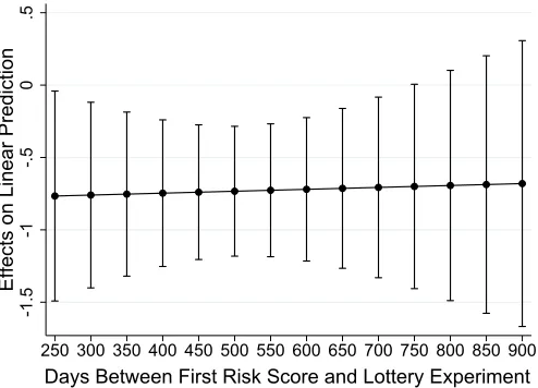
effect between the subjective response and the days since the response was given (Figure
6).
As Figure6shows, the marginal effect of subjective risk preferences on an individual’s
lottery choice is always around -0.7. The relationship is statistically significant at the .05
level for responses given up to 2 years prior. After that point, we simply do not have enough
observations to show the correlation with any confidence.
Naturally, it may be that the statistically significant relationship between subjective
risk preferences and decisions made in the incentivized lottery experiment is being driven
only by workers who participated in more than one experiment. This would be troublesome
because it could suggest that only the decisions made by workers who participate in more
than one experiment are economically relevant. Given that workers who participate in
more than one experiment tend to be older, less willing take risk, and less impulsive
-this seems like a reasonable possibility. To explore whether or not -this is the case, we
Figure 6: Marginal Effect of Willingness to Take Risk as Number of Days Since 1st Response Increases.
-1.
5
-1
-.5
0
.5
Ef
fect
s
on
Linear
Predict
ion
250 300 350 400 450 500 550 600 650 700 750 800 850 900
Days Between First Risk Score and Lottery Experiment
Marginal effect estimated from Model 4 in Table3. Bars represent 95% confidence intervals.
experiment (EXP=1) and workers who participate in more than one experiment (EXP>1).
These results are presented in Table4.
The results presented in Table4suggest that the subjective risk preferences of workers
who participate in only one experiment predict risky decision making in the real stakes
experiment. Further, coefficients in the models that use data from workers who completed
only a single experiment are in the same ballpark as counterparts presented in Table 3as
well as models that use data from workers who completed more than one experiment.
In all, the results in this section are an important indication that AMT workers give not
only consistent responses, but responses that map onto actual behavior. Further, because
the responses are consistent, it does not matter when the response was recorded. Responses
taken several months prior are just as good at predicting risky behavior in a real stakes task
as responses taken at the same time. This suggests that, on average, AMT workers provide
Table 4: Subjective Risk Preferences and Risky Decision Making in a Real Stakes Task (Group 1 vs Group 2)
Model 1 Model 2 Model 3 Model 4
EXP=1 EXP>1 EXP=1 EXP>1
Coef. S.E Coef. S.E Coef. S.E Coef. S.E
Contemporaneous Risk -0.573 0.192 -0.605 0.242 -0.493 0.25 -0.588 0.245
Male 1.077 1.208 2.175 1.324
Age 0.006 0.046 0.096 0.053
Impulsivity -0.059 0.06 0.076 0.06
Constant 14.756 1.093 14.025 1.291 17.426 3.349 4.765 5.495
Obs 69 53 66 53
R2 0.0211 0.0194 0.0257 0.0393
LL 5 4 4 4
UL 1 1 1 1
Tobit models. The dependent variable is the index number of lottery selected: larger values indicate less risky choices. LL(UL) indicates the number of workers who selected lottery 1(20).
5 Discussion and Conclusion
Critics of studies using Amazon Mechanical Turk question the validity of studies using the
platform for a wide variety of reasons. Many of these criticisms are valid. Namely,
ex-periments involving an element of social interaction or those that require specific subject
pools/samples are probably not best suited for the platform. However, in many
experi-ments, these types of criticism are not applicable. Therefore, the primary concerns become
those related to consistency and economic relevancy of workers’ responses. We show that
workers on Amazon Mechanical Turk consistently report their basic demographics,
subjec-tive risk preferences, and impulsivity. Further, their responses are economically relevant
in, at the very least, a basic lottery experiment. Subjective willingness to take risk is
signif-icantly correlated with behavior in an incentivized lottery experiment and in the direction
one would expect. In sum, the results suggest the quality of data obtained via AMT is not
are recorded.
Researchers need to, however, use Amazon Mechanical Turk with care. AsArechar
et al. (2017) shows, the population completing tasks on Amazon Mechanical Turk tends
to be more male during the weekdays and the studies used to generate the data set that
is analyzed here support this finding. Researchers using AMT should provide the time the
HIT was posted along with any observed differences in their samples from ongoing large
scale projects. Further, while the population of workers is generally more representative
of the US population than typical university subject pools, there are still significant
differ-ences between the worker population and US population. Researchers need to take these
differences seriously before making external validity claims. In terms of future steps,
nor-matively, research using AMT is lacking in standardization. Unlike the lab, there are few
established norms for conducting research on AMT or online, generally. A consensus of
best practices (e.g., pay and reasons for blocking workers) needs to be reached for
com-parisons across studies to be meaningful. Such standardization could also foster increased
experimental control.
To close, there are three caveats regarding the results presented in this manuscript.
First, this paper is not about the overall demographics of the AMT worker population.
Worker demographics vary across the day and week and there is evidence of long term
trends in changing demographics. Given that the experiments were posted during
rela-tively consistent times of day and over a long period of time, there is no reason to believe
that the demographics presented will match the demographics of today’s AMT worker
pop-ulation. Indeed, they do not. Second, this paper is not about identifying the inter-temporal
correlation of various worker characteristics and demographics under the most controlled
conditions allowed in the environment. The experiments from which we include data vary
widely and the order of the measures taken in the experiments do as well. Further, we try to
provided inconsistent answers, did not complete the experiment, or failed an English
com-prehension/attention check question.16 Third, it is well-known that the population of AMT
workers may not be suitable for all research questions. While it is true that,
demograph-ically, AMT workers are significantly more varied than university subject pools (Ipeirotis,
2010;Buhrmester et al.,2011;Behrend et al.,2011), the AMT population is not
represen-tative of the US population as a whole. American workers on AMT generally have a lower
reported income than the overall population of the US (c.f.,Paolacci et al.,2010; Berinsky
et al.,2012; Levay et al.,2016), are more likely to report to be unemployed (e.g.,
Ipeiro-tis,2010;Goodman et al.,2016), younger, and are more ideologically liberal (Berinsky et
al., 2012).17 Thus, this paper is not arguing that AMT is a suitable tool for all research
questions. Instead, as we have shown, the purpose of this paper is to demonstrate that
even in inconsistent settings, with low stakes, in an uncontrolled environment, with some
of the worst workers possible, workers on AMT can provide consistent and economically
meaningful data.
16So in some sense, the data analyzed in this study is the experimentalist’s worst
night-mare.
17However, AMT workers are fairly similar to samples created using other online survey
References
Arechar, Antonio A, Gordon T Kraft-Todd, and David G Rand (2017) ‘Turking Overtime:
How Participant Characteristics and Behavior Vary Over Time and Day on Amazon
Me-chanical Turk.’Journal of the Economic Science Association3(1), 1–11
Behrend, Tara S, David J Sharek, Adam W Meade, and Eric N Wiebe (2011) ‘The Viability
of Crowdsourcing for Survey Research.’Behavior research methods43(3), 800
Benjamini, Yoav, and Yosef Hochberg (1995) ‘Controlling the False Discovery Rate: A
Prac-tical and Powerful Approach to Multiple Testing.’Journal of the Royal Statistical Society,
Series B (Methodological)57(1), 289–300
Berinsky, Adam J, Gregory A Huber, and Gabriel S Lenz (2012) ‘Evaluating Online Labor
Markets for Experimental Research: Amazon.com’s Mechanical Turk.’ Political Analysis
20(3), 351–368.
Buhrmester, Michael, Tracy Kwang, and Samuel D Gosling (2011) ‘Amazon’s Mechanical
Turk: A New Source of Inexpensive, Yet High-Quality, Data?’ Perspectives on Psychological
Science6(1), 3–5
Carlin, Ryan E., and Gregory J. Love (2013) ‘The Politics of Interpersonal Trust and
Reci-procity: An Experimental Approach.’Political Behavior35(1), 43–63
Clifford, Scott (2014) ‘Linking issue stances and trait inferences: a theory of moral
exem-plification.’The Journal of Politics76(3), 698–710
Clifford, Scott, and Ben Gaskins (2016) ‘Trust Me, I Believe in God: Candidate Religiousness
as a Signal of Trustworthiness.’American Politics Research44(6), 1066–1097
Converse, Philip E. ‘Information flow and the stability of partisan attitudes.’Public Opinion
Dave, Chetan, Catherine C. Eckel, Cathleen A. Johnson, and Christian Rojas (2010)
‘Elicit-ing Risk Preferences: When is Simple Better?’ Journal of Risk and Uncertainty41(3), 219–
243
Del Ponte, Alessandro, Andrew W. Delton, Reuben Kline, and Nicholas A. Seltzer (2017)
‘Passing It Along: Experiments on Creating the Negative Externalities of Climate Change.’
Journal of Politics79(4), 1444–1448
Dohmen, Thomas, Armin Falk, David Huffman, Uwe Sunde, Jürgen Schupp, and Gert G
Wagner (2011) ‘Individual Risk Attitudes: Measurement, Determinants, and Behavioral
Consequences.’Journal of the European Economic Association9(3), 522–550.
Farrington, David P. (1998) ‘Predictors, Causes, and Correlates of Male Youth Violence.’
Crime and Justice24, 421–475
Flores, Andrew R, Taylor NT Brown, and Jody Herman (2016)Race and Ethnicity of Adults
Who Identify as Transgender in the United States(Williams Institute, UCLA School of Law)
Fowler, James H., and Cindy D. Kam (2007) ‘Beyond the Self: Social Identity, Altruism, and
Political Participation.’The Journal of Politics69(3), 813–827
Gibson, John, and David Johnson (2018) ‘Assessing the Stability of Risk Preferences Online.’
Technical Report, University of Central Missouri
Goodman, Joseph K., Cynthia E. Cryder, and Amar Cheema (2013) ‘Data Collection in
a Flat World: The Strengths and Weaknesses of Mechanical Turk Samples.’ Journal of
Behavioral Decision Making26(3), 213–224
Goodman, William K, Ashley M Geiger, and Jutta M Wolf (2016) ‘Differential Links
be-tween Leisure Activities and Depressive Symptoms in Unemployed Individuals.’Journal
Hatemi, Peter K., John R. Alford, John R. Hibbing, Nicholas G. Martin, and Lindon J. Eaves
(2009) ‘Is There a ’Party’ in Your Genes?’ Political Psychology(3), 584–600
Holt, Charles A, and Susan K Laury (2002) ‘Risk Aversion and Incentive Effects.’American
economic review92(5), 1644–1655.
Horton, John J, David G Rand, and Richard J Zeckhauser (2011) ‘The Online Laboratory:
Conducting Experiments in a Real Labor Market.’ Experimental Economics 14(3), 399–
425
Huff, Connor, and Dustin Tingley (2015) ‘“Who are These People?” Evaluating the
Demo-graphic Characteristics and Political Preferences of MTurk Survey Respondents.’Research
& Politics2(3), 2053168015604648
Ipeirotis, Panagiotis G (2010) ‘Demographics of Mechanical turk.’
Johnson, David B, and Matthew D Webb (2016) ‘Decision Making with Risky, Rival
Out-comes: Theory and Evidence.’ Technical Report, Carleton University, Department of
Eco-nomics
Krupnikov, Yanna, and Adam Seth Levine (2014) ‘Cross-Sample Comparisons and External
Validity.’Journal of Experimental Political Science1(1), 59–80
Levay, Kevin E, Jeremy Freese, and James N Druckman (2016) ‘The Demographic and
Po-litical Composition of Mechanical Turk Samples.’SAGE Open6(1), 2158244016636433.
Lopez, Jesse, and D. Sunshine Hillygus (2018) ‘Why So Serious?: Survey Trolls
and Misinformation.’ Available at SSRN: https://ssrn.com/abstract=3131087 or
http://dx.doi.org/10.2139/ssrn.3131087
Self-Regulation and Self-Exploration in the Life Stories of Religious American Conservatives
and Liberals.’Political Pyschology34(2), 201–219
McDermott, Rose, Chris Dawes, Elizabeth Prom-Wormley, Lindon Eaves, and Peter K.
Hatemi (2013) ‘MAOA and Aggression: A Gene–Environment Interaction in Two
Pop-ulations.’The Journal of Conflict Resolution57(6), 1043–1064
Milita, Kerri, Elizabeth N. Simas, John Barry Ryan, and Yanna Krupnikov (2017) ‘The Effects
of Ambiguous Rhetoric in Congressional Elections.’Electoral Studies46(April), 48–63
Mullinix, Kevin J., Thomas J. Leeper, James N. Druckman, and Jeremy Freese (2015)
‘The Generalizability of Survey Experiments.’ Journal of Experimental Political Science
2(2), 109–138
Paolacci, Gabriele, Jesse Chandler, and Panagiotis G Ipeirotis (2010) ‘Running Experiments
on Amazon Mechanical Turk.’
Richter, David, Julia Roher, Maria Metzing, Wiebke Nestler, Michael Weinhardt, and Jürgen
Schupp (2017) ‘SOEP Scales Manual (updated for SOEP-Core v32. 1).’ Technical Report,
SOEP Survey Papers
Stanford, Matthew S, Charles W Mathias, Donald M Dougherty, Sarah L Lake, Nathaniel E
Anderson, and Jim H Patton (2009) ‘Fifty Years of the Barratt Impulsiveness Scale: An
Update and Review.’Personality and Individual Differences47(5), 385–395
Verkoeijen, Peter P. J. L., and Samantha Bouwmeester (2014) ‘Does Intuition Cause
Coop-eration?’ PloS ONE. https://doi.org/10.1371/journal.pone.0096654
Zaller, John (1992)The Nature and Origins of Mass Opinion(New York: Cambridge
Appendix for:
Amazon Mechanical Turk Workers Can Provide
Consistent and Economically Meaningful Data
June 28, 2018
1 Day of the Week
[image:30.612.114.482.384.645.2]Figure A.1 presents the percentage of workers who report to be male, their average age, average willingness to take risk, and average Impulsiveness Test scores by the day of the week.
Figure A.1: Gender, Age, Risk, and IMP by Day of Week
0
.2
.4
.6
Percent Male
Sun. Mon. Tue. Wed. Thu. Fri. Sat.
Day of the Week
0
10
20
30
40
Age
Sun. Mon. Tue. Wed. Thu. Fri. Sat.
Day of the Week
0
2
4
6
Risk
1
Sun. Mon. Tue. Wed. Thu. Fri. Sat.
Day of the Week
0
20
40
60
IMP
1
Sun. Mon. Tue. Wed. Thu. Fri. Sat.
Day of the Week
Notes: First/only reported gender, age, willingness to take risk, and Barratt Impulsivity
2 Determinants of the Number of Experiments Completed
[image:31.612.133.462.208.363.2]Table B.1 presents the primary Pearson correlations of the variables of interest and the number of experiments the worker completed (Completions). The correlations, in terms of characteristics and the number of experiments completed, generally fall into the direction one would expect: workers who are more willing to take risk completed fewer experiments and tend to be more impulsive.
Table B.1: Correlations of Main Variables
Completions Male1 Age1 Risk1
Male1 0.0508
(0.001)
Age1 0.0367 -0.1568
(0.051) (<0.001)
Risk1 -0.0596 0.1632 -0.1287 (<0.001) (<0.001) (<0.001)
IMP1 -0.0819 0.0505 -0.1287 0.2155
(<0.001) (0.009) (<0.001) (<0.001)
Notes: Correlations of primary variables of interest and the
3 Gender Differences
There are some interesting gender differences to report. These differences are summarized in TableC.1. First, when examining all workers’ first/only responses, we find that males are significantly more impulsive and more willing to take risk. While the significant difference in willingness to take risk is consistent with prior studies (c.f., Dohmen et al., 2011) the difference in impulsiveness is not. However, our reported difference is small in magnitude and consistent with the magnitude of the difference reported inStanford et al.(2009) that was not found to be statistically significant (62.8 vs 62.1). Second, females are significantly older.
The difference in average ages across genders is important to highlight because previ-ous literature has identified an inverse relationship between impulsiveness and ageSpinella
[image:32.612.189.404.413.641.2](c.f.,2007). Thus, given that females in the sample are significantly older it is reasonable to expect them to be less impulsive. To further address the impulsiveness discrepancy, we use OLS to estimate workers’ first/only impulsiveness test score (Obs= 1, 377) using first reported gender and age as independent variables. The OLS results support the above proposition as the coefficient on age is found to be statistically significant (coef=-0.151, p< 0.001) while gender (1 if male; 0 if female) is not (coef=0.079, p =0.904). Finally, when examining workers’ second responses, the gender difference in impulsiveness is no longer significant while the significant differences in age and risk remains. These results are available upon request.
Table C.1: Gender Differences
First Response (All workers)
IMP Risk Age
Male 60.533 5.678 31.230
Female 59.346 4.779 34.401
t-test: 0.009 <0.001 <0.001 u-test: 0.004 <0.001 <0.001
Second Responses
IMP Risk Age
Male 58.365 5.259 32.959
Female 58.260 4.338 35.792
t-test: 0.971 <0.001 0.004 u-test: 0.661 <0.001 0.007
Notes: Gender differences in
4 Consistency of Individual Test Questions
Table D.1: Differences in Each Impulsiveness Test Question
IMPQ1,2 IMPQ2,2 Diff p B.H.p r
I plan tasks carefully. 3.054 3.135 -0.081 0.028 0.757 0.493
I do things without thinking. 1.611 1.616 -0.005 0.896 1.000 0.481
I make-up my mind quickly. 2.377 2.374 0.002 0.953 1.000 0.459
I am happy-go-lucky. 2.328 2.328 0 1.000 1.000 0.672
I don’t pay attention. 1.387 1.397 -0.01 0.778 1.000 0.444
I have racing thoughts. 1.958 1.958 0 1.000 1.000 0.471
I plan trips well ahead of time. 3.039 3.086 -0.047 0.247 0.926 0.539
I am self controlled. 3.064 3.069 -0.005 0.898 1.000 0.484
I concentrate easily. 2.966 3.005 -0.039 0.292 0.9733 0.579
I save regularly. 2.766 2.8 -0.034 0.397 1.000 0.651
I squirm at plays or lectures. 1.988 2.057 -0.069 0.101 0.758 0.6
I am a careful thinker. 3.128 3.153 -0.025 0.516 1.000 0.49
I plan for job security. 2.761 2.781 -0.02 0.637 1.000 0.599
I say things without thinking. 1.707 1.707 0 1.000 1.000 0.46
I like to think about complex problems. 2.736 2.736 0 1.000 1.000 0.603
I change jobs. 1.756 1.707 0.049 0.208 0.891 0.493
I act on impulse. 1.8 1.8 0 1.000 1.000 0.435
I get easily bored when solving thought problems. 1.862 1.865 -0.002 0.954 1.000 0.439
I act on the spur of the moment. 1.877 1.872 0.005 0.902 1.000 0.467
I am a steady thinker. 3.012 3.079 -0.067 0.077 0.758 0.523
I change residences. 1.638 1.65 -0.012 0.745 1.000 0.505
I buy things on impulse. 1.842 1.842 0 1.000 1.000 0.475
I can only think about one thing at a time. 1.906 1.906 0 1.000 1.000 0.519
I change hobbies. 1.84 1.818 0.022 0.574 1.000 0.502
I spend or charge more than I earn. 1.562 1.554 0.007 0.838 1.000 0.585
I often have extraneous thoughts when thinking. 2.135 2.081 0.054 0.194 0.891 0.515
I am more interested in the present than the future. 2.357 2.337 0.02 0.631 1.000 0.497
I am restless at the theatre or lectures. 1.929 1.988 -0.059 0.156 0.891 0.604
I like puzzles. 2.951 2.879 0.071 0.072 0.758 0.616
I am future oriented. 2.754 2.761 -0.007 0.857 1.000 0.55
Notes: First (IMPQ1,2) and last (IMPQ2,2) impulsiveness test question and difference in
5 The Experiments
[image:35.612.68.533.166.520.2]In TableE.1, we present the eleven experiments that we used to generate the data set. A brief description of each of the experiments is given in the subsections below.
Table E.1: The Experiments
Age Gender Risk IMP Start Date
Study 1
Ø Ø Ø Sept 12, 2012
(Obs=865) Study 2
Ø Ø Feb 17, 2014
(Obs=235) Study 3
Ø Ø Ø Ø Mar 14, 2015
(Obs=485) Study 4
Ø Ø Ø Ø May 11, 2015
(Obs=314) Study 5*
Ø Ø Ø Feb 26, 2016
(Obs=60) Study 6*
Ø Ø Ø Mar 16, 2016
(Obs=504) Study 7*
Ø Ø Ø Apr 26, 2016
(Obs=250) Study 8
Ø Ø Ø Ø Jul 08, 2016
(Obs=649) Study 9
Ø Ø Ø Mar 23, 2017
(Obs=970) Study 10
Ø Ø Ø Nov 26, 2017
(Obs=940) Study 11
Ø Ø Ø Ø Jan 17, 2018
(Obs=75)
Notes: Experiments in the data set. Left most column indicates the authors of the
HIT/study and the number of submissions (Obs). Middle four columns indicate the ques-tions that are asked in the study. Final column indicates the first day a batch of the exper-iment was posted. “*” indicates that the study was joint work with a student for a school project. All studies were approved by the IRB of the University the first author was affiliated with at the time of the study.
5.1 Ambiguity and Performance Pay (Study 1)
categories. In the transcription task, workers were shown an image of a word and had to type the word that was shown into a text box. The experiment varied the information given to workers relating to how their bonuses were calculated if they selected the coding task and the amount they would be paid if they completed the transcription task. Workers reported their age, gender, and willingness to take risk in a survey that occurred prior to the main experiment. Workers on average earned about $0.60 and spent about 15 minutes on the experiment.
5.2 The Effect of Financial Goals and Incentives on Labor. An Experimental Test in
a Real(ish) Labor Market (Study 2)
In the experiment, workers were assigned into one of four treatments and completed a real effort task. Workers transcribed pieces of an instruction manual from a 1996 Oldsmobile Cutlass. Before seeing the treatment screen, workers completed five practice transcriptions, each paying 2 cents each. In the treatment assignment screen, which was shown after the practice period, workers read a short piece of text that assigned them to a treatment and gave them a wage rate. In the “Do Your Best” treatment, the text read “Working for us your goal is to just do your best and do as many sentences as you can” in the “goal” treatment, the text read “Working for us your goal is to make $2.” Above this information, workers were shown their wage rate that would be paid (2 Cents or 5 Cents). Workers were paid this amount for each transcription they completed. Workers reported their age and gender prior to the treatment assignment screen. Workers, on average, made a little more than $2 dollars and spent about 30 minutes on the task. While workers in this study also completed the Barratt Impulsiveness Test after the experiment, one of the question responses had the same name as a different question. Thus, responses to this question were overwritten. Therefore, we do not use Impulsiveness test scores from this study.
5.3 An Experimental Test of the No Safety Schools Theorem (Study 3)
Table E.2: Lotteries Used in the Experiments
A B C D E F G H I J K L M N O P Q R S T
Prob .05 .10 .15 .20 .25 .30 .35 .40 .45 .50 .55 .60 .65 .70 .75 .80 .85 .90 .95 1.00
Prize 5.00 4.75 4.50 4.25 4.00 3.75 3.50 3.25 3.00 2.75 2.50 2.25 2.00 1.75 1.50 1.25 1.00 0.75 0.50 0.25
EV 0.25 0.48 0.68 0.85 1.00 1.13 1.23 1.30 1.35 1.38 1.38 1.35 1.30 1.23 1.13 1.00 0.85 0.68 0.48 0.25
Notes: Lotteries used in Study 3 and Study 11.
5.4 Untitled Stress Experiment (Study 4)
This experiment explored the effect of quickly shown images on productivity. Productivity was measured using a real effort task. Workers were assigned into one of three groups. In the treatment groups, after completing 4 real effort tasks, workers were shown either an image of a seal or Linda Blair (in full exorcist make-up). In the control group, workers were not shown any image. Age and gender were collected prior to the start of the main experiment. Impulsivity and willingness to take risk were collected after.
5.5 Testing for Selection on AMT (Study 5)
Workers who accepted the HIT were assigned into one of two treatments. In the first treat-ment, workers completed a survey on AMT. In the second treattreat-ment, workers completed the same survey but had to click a link that took them to the same survey that was hosted on Survey Monkey instead of AMT. The experiment paid $1.50 and workers spent, on average, about 30 minutes on the experiment. Because workers who were assigned to the treatment that had them complete the survey on Survey Monkey did not have their Worker ID number attached to their answers, we us only workers who participated in the first treatment.
5.6 The Effect of Differential Tuition on Choice of College Major (Study 6)
5.7 The Effect of Precision Pricing on Perceived Home Value (Study 7)
This experiment explored the effect of “precision pricing” on the amount workers would be willing to bid on homes. In the experiment, workers were shown a set of three homes. The experiment varied the type of homes (low cost vs high cost) workers bid on (110,000 and 300,000) and the precision of the price (house value+.05%,+0, and -.05% of the home’s value). Workers were paid 1 dollar for participating and the experiment took on average 36 minutes. The survey, which collected workers’ age, gender, and impulsivity, took place after the experiment.
5.8 The Effect of Wage Inequality (Study 8)
This experiment explored the interaction of pay and knowledge of others’ pay on worker productivity. Workers in the experiment were paid either 2, 4, or 20 cents for each word they correctly coded and were truthfully told some other workers are paid 2, 4 or 20 cents for each word they correctly code. To identify wage effects, some workers were given no information regarding the wage rates of others. After completing the real effort portion of the experiment, workers completed the survey. Workers on average earned $1.85 and took 32 minutes to complete the experiment. Age and gender was collected prior to the start of the experiment. Impulsivity and willingness to take risk was collected after.
5.9 Should I Give up or Hold out? The Differential Impact of Debt on Wage Selectivity
I (Study 9)
In the experiment presented in this paper, workers participated in a two period experiment. In the first period workers were assigned a debt (that was randomly assigned) and given a “wage” offer. Workers then decided whether to reject or accept the wage offer. If the worker accepted the wage offer, the worker earned two times the offered wage (from working both periods) minus their assigned debt. If the wage offer was rejected, the worker was given a second wage offer and earned the second wage minus their assigned debt. If the worker ended the experiment with negative earnings, the worker earned nothing. On average, the experiment took 7.6 minutes to complete and paid $0.26 in addition to a $0.25 participation fee. Age, gender, risk, and impulsivity were all collected prior to the start of the experiment.
5.10 Should I Give up or Hold out? The Differential Impact of Debt on Wage
Selec-tivity II (Study 10)
to a $0.25 cents participation fee. Age, gender, risk, and impulsivity were all collected prior to the start of the experiment.
5.11 The Economic Relevancy of Risk Preferences Elicited Online and With Low
Stakes (Study 11)
In the experiment presented in this paper, workers completed a set of surveys and four risk aversion tests with monetary incentives. On average, workers spent 18 and a half minutes on the experiment and earned $4.39. Age and gender was collected prior to the start of the first two risk aversion tests (a standard Holt and Laury and a Holt and Laury with 15 stakes -Holt and Laury(2002)). Risk and impulsivity was collected after completing the first two risk aversion tests but before the final two risk aversion tests (Gneezy and Potters,1997;
Johnson and Webb,2016).
References
Benjamini, Yoav, and Yosef Hochberg (1995) ‘Controlling the False Discovery Rate: A Prac-tical and Powerful Approach to Multiple Testing.’Journal of the Royal Statistical Society, Series B (Methodological)57(1), 289–300
Charness, Gary, and Martin Dufwenberg (2006) ‘Promises and partnership.’Econometrica 74(6), 1579–1601
Dohmen, Thomas, Armin Falk, David Huffman, Uwe Sunde, Jürgen Schupp, and Gert G Wagner (2011) ‘Individual Risk Attitudes: Measurement, Determinants, and Behavioral Consequences.’Journal of the European Economic Association9(3), 522–550.
Gneezy, Uri, and Jan Potters (1997) ‘An Experiment on Risk Taking and Evaluation Periods.’ The Quarterly Journal of Economics112(2), 631–645
Holt, Charles A, and Susan K Laury (2002) ‘Risk Aversion and Incentive Effects.’American economic review92(5), 1644–1655.
Johnson, David B, and Matthew D Webb (2016) ‘Decision Making with Risky, Rival Out-comes: Theory and Evidence.’ Technical Report, Carleton University, Department of Eco-nomics
Spinella, Marcello (2007) ‘Normative Data and a Short Form of the Barratt Impulsiveness Scale.’International Journal of Neuroscience117(3), 359–368