http://dx.doi.org/10.4236/am.2013.41003 Published Online January 2013 (http://www.scirp.org/journal/am)
A Modified Homotopy Analysis Method for Solving
Boundary Layer Equations
Yinlong Zhao, Zhiliang Lin, Shijun Liao
School of Naval Architecture, Ocean and Civil Engineering, Shanghai Jiao Tong University, Shanghai, China Email: [email protected]
Received October 28, 2012; revised November 28, 2012; accepted December 4, 2012
ABSTRACT
A new modification of the Homotopy Analysis Method (HAM) is presented for highly nonlinear ODEs on a semi-infi- nite domain. The main advantage of the modified HAM is that the number of terms in the series solution can be greatly reduced; meanwhile the accuracy of the solution can be well retained. In this way, much less CPU is needed. Two typi-cal examples are used to illustrate the efficiency of the proposed approach.
Keywords: Homotopy Analysis Method; Boundary Layer Equations; Orthonormal Functions
1. Introduction
In 1992, Liao [1] proposed the Homotopy Analysis Me- thod (HAM) to solve nonlinear differential equations analytically. Since then, HAM has been used to investi- gate a variety of mathematical and physical problems [2]. As is well known, HAM has the advantage of indepen- dence on small physical parameters and adjusting the convergence region and convergence rate of the series solution over perturbation method. However, for some type of auxiliary operator (i.e. base functions), it is usual- ly time-consuming to get high-order approximation, and the number of terms appearing in high order approxima- tion is very huge.
To improve the efficiency of HAM, many scholars have proposed different techniques. Yabushita [3] suggested an optimal HAM approach by minimizing the residual of governing equations. Marinca [4], Niu [5], Liao [6] de- veloped this kind of approach. Lin [7] suggested an itera- tive technique, in which the initial guess is continuously replaced by intermediate approximation to proceed the computation. Recently, we use orthonormal polynomials/ functions to approximate the right-hand side of the high- order deformation equations to prohibit the rapid growth of the terms appearing in approximate solutions. For dif- ferential equations defined on a finite interval, trigono- metric functions (or polynomial functions) are usually selected to express solutions. In this case, orthonormal trigonometric functions (or Chebyshev polynomials) are used to approximate right-hand side of high-order de- formation equations. In this paper, we generalize this kind of approach for nonlinear problems defined on semi-infinite intervals. The main idea is that orthonormal
functions derived from Schmidt-Gram process are used to approximate the right-hand side of high-order defor- mation equations during computation. For different types of problems, the derived orthonormal functions are dif- ferent, which are closely related to the solution expres- sion.
In the following section, the modified HAM (MHAM) is presented for boundary layer problems. In Section 3, examples are given to demonstrate it. Conclusions and some discussions are given in the last section.
2. Analysis of the Method
For convenience, a brief description of the standard HAM will be present first. Then the proposed truncation tech- nique will be followed.
Without loss of generality, consider the differential equation
0N u t , (1) where N is a nonlinear operator, t denotes the independ- ent variable, u t
is an unknown function. Suppose
u t could be expressed by a set of functions
k t k0 (2) such that
0
k k k
u t a t
(3)is uniformly valid, where kis a coefficient. In HAM, the zeroth-order deformation equation is constructed as
a
where
0
; m m
m
t q u t q
, (5)L is an auxiliary linear operator, and H t
the aux- iliary function. Applying the homotopy-derivative [8]
0
1 !
m
m m
q
D
m q
(6)
to both sides of Equation (4), we get the corresponding mth-order deformation equation
1
0
1,m m m m
L u t u t c H t R m1, (7) where
1 1 ;
m m
R D N t q , (8) and
0, 1, 1, 1. m
m m
(9) Note that 1 2 can be obtained by solving linear Equation (7) one after the other. The mth-order appro- ximation of is given by
, , u u
u t
0
m m
k
U
uk (10)To measure the accuracy of m, the squared residual error for Equation (1) is defined as
U
2 d m A N Um t
, where A is the domain.If a successful homotopy analysis solution is obtained, the difficulty to get better approximation is that with the growth of order, the number of terms in higher-order ap- proximation will grow rapidly, resulting in an enormous amount of computing time. To address this problem, we propose a truncation technique. The basic idea is that the right-hand side of Equation (7) is approximated by a set of orthonormal functions.
Suppose that m1 can be expressed by a finite linear combination of linearly independent functions
R
k t
,
. Note that
1, 2,
k k
may be slightly different from
k . Define a proper inner product in the linear space spanned by 1, 2,,N as
,
A d
f g
t f t g t t, (11) where is a weight function. In the framework of HAM, two typical kinds of base functions are usually used for boundary layer problems.
t Case 1: suppose that m1 can be expressed by finite linear combination of linearly independent functions
R
tnem t n0,m1,
Note that (12) is dependent on three parameters , m and n. To implement the orthonormalization, an order is given to (12) as follows (called triangular order):
1 1
2
e
n m t
m n m n n
t
.
The inner product is defined as
f g,
0f t g t
d .tCase 2: suppose that Rm1 can be expressed by finite linear combination of linearly independent functions
t n n0,1
. (13) The inner product is defined as
f g,
1f t g t
dt. (14) Applying the Schmidt-Gram process to the first functionsN
1
,2,, N , we obtain orthonormal functions 1 2
N
, , , N
e e e . Every time when Rm1 is got, we approximate it by e e1, 2, , N
N e
, to ensure that the number of terms in the right-hand side of Equation (7) will be no more than . That is to say, we replace
1
m
R with its approximation
1 1
,
N
m m i
i
R R e
i
e (15)
to proceed the computation in HAM.
3. Numerical Experiment
To illustrate the efficiency of the truncation technique, two typical examples are considered. The codes are writ-ten in Maple 13 on a PC with an Intel Core 2 Quad 2.66 GHz CPU. The variable Digits in the experiments is to control the number of digits when calculating with soft-ware floating point numbers in Maple.
3.1. Example 1
Let us consider the Blasius Equation (9)
1
0 2
f f f , (16) subject to the boundary conditions
0
0 0,
f f f 1, (17) where the prime denotes the derivative with respect to . Following Liao [9], we seek the solution f
in the form
0,0 ,1 0
e
n m
m n
m n
f a a
,where 0 is the spatial-scale parameter, and m n, is a coefficient. The auxiliary linear operator is chosen as
a
3
3 2
2; ;
; q q
L q
.
The initial guess is
0
1 e
f
.
The zeroth-order deformation equation is constructed as in (4), and the th-order deformation equation as in (7) with homogeneous boundary conditions
m
0
0
0,m m m
f f f m1, where
1
1 1 1
0
1 2
m
m m k m k
k
R f f f
.For this example, the first kind orthonormal functions are used to approximate Rm1 every time when Rm1 is got. Then Rm1 is used to compute fm instead of
. In the experiment, we set 1
m
R 4, ,
, and
36
N
100
s
Digit H 1. From Tables 1 and 2, we can see that though we use approximate Rm1 (i.e. Rm1) to do the computation, the residual error m and f
0 given by MHAM are almost the same as that given by standard HAM. From Table 3, we can see that the num- ber of terms in high-order approximation given by MHAM is 39, while that given by HAM grows exponen- tially. Moreover, it shows that MHAM needs less than ninth the CPU time used by HAM to get 50th-order ap- proximate solution. The curve of residual error and CPU time is plotted in Figure 1. From it we can see that the truncation technique greatly improves the efficiency of HAM.3.2. Example 2
Consider a set of two coupled nonlinear differential equa- tions (see Kuiken [10] for details)
2
0
f f (18)
3 f
(19) with the boundary conditions
0
0f f 0,
0 1, f
0, where is the Prandtl number.Under the transformation
1
, F
f
, Equations (18) and (19) become
2F S F2 0
, (20)
2
3
S F S
[image:3.595.68.251.86.162.2] , (21) with the boundary conditions
Table 1. Comparison of f
0 given by MHAM and HAM in Example 1.Order m MHAM HAM
10 0.3277556 0.3277556
20 0.3318513 0.3318513
30 0.3320404 0.3320403
40 0.3320557 0.3320555
[image:3.595.308.537.117.207.2]50 0.3320573 0.3320571
Table 2. Comparison of given by MHAM and HAM in Example 1.
m
δ
Order m MHAM HAM
10 1
1.9500 10 1
1.9500 10
20 3
3.8793 10 3
3.8793 10
30 4
1.1616 10 4
1.1616 10
40 6
3.9192 10 6
3.9192 10
50 7
1.4013 10 7
1.4008 10
Table 3. Comparison of CPU time (seconds) and number of terms appearing in mth order approximation given by MHAM and HAM in Example 1.
MHAM HAM
Order m
Terms Time (sec) Terms Time (sec)
10 39 49.530 123 0.791
20 39 103.837 443 9.52
30 39 158.952 963 72.832
40 39 215.133 1683 537.956
50 39 271.667 2603 2488.035
10-1
10-3
10-5
10-7
10-9
MHAM HAM
Er
r
0 500 1000 1500 2000 2500 CPU (s)
[image:3.595.307.540.394.708.2] [image:3.595.307.540.396.718.2]
1 0F , S
1 1, F
S
0.We seek the solutionF
andS
in the form
2
n n n
F a
,
4 n n nS b
,where n, n are coefficients.
Following Liao [2], the auxiliary linear operators are chosen as a b 2 2 3 F L , 2 2 5 S L
and the initial guess of F
and S
as
2 3
0F ,
4 0S . Then the high-order deformation equations become
1
1F
F n n n F F
L F F c H Rn
0
,
1
1S
S n n n S S n
L S S c H R , subject to the homogeneous boundary conditions
1
1
n n n n
F S F S , and
1
2
1 1 1 1
0
n F
n n n j n j
j
R F S F F
,
1
2
1 1 1
0
3
n S
n n j n j
j
R S F S
.We find that 1
F
n and n 1
R RS
can be expressed in the
form of finite combination of functions
n n4
, (22) and
n n6
, (23) respectively. Applying the Schmidt-Gram process to the first functions in (22) and (23), respectively, we ob- tain two set of N orthonormal functions, denoted by
N
F e and S. We use
e eF to approximate F1 n
R every time it is got, and to approximate 1. Then
S
e RnS RnF1 and 1
S n
R are used to proceed the computation.
In the experiment, we set N15, 1, 1 3,
1 2
F S
c c , , and D . For
different order approximation given by the two app- roaches, the quantity is showed in Table 4, and the residual error for Equation (20) is compared in Table 5. We can see that although we use
1
F S
H H
0f
igits
1
100
F n
R to proceed the computation instead of 1
F n
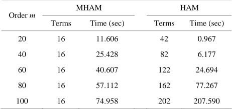
[image:4.595.309.540.115.214.2]R , the accuracy of the app- roximate solution is well retained. From Table 6, we can see that the number of terms in the high-order approxi- mation given by MHAM was kept within 16, while that
Table 4. Comparison of f
0 given by MHAM and HAM in Example 2.Order m MHAM HAM
20 0.6971702145 0.6971702149
40 0.6932675852 0.6932675846
60 0.6932116278 0.6932116273
80 0.6932116054 0.6932116060
[image:4.595.307.539.241.328.2]100 0.6932116316 0.6932116326
Table 5. Comparison of given by MHAM and HAM in Example 2.
m
δ
Order m MHAM HAM
20 5
1.4233 10 5
1.4233 10
40 9
4.3708 10 9
4.3708 10
60 12
8.9385 10 12
1.1883 10
80 13
6.0625 10 13
5.9355 10
100 14
9.7190 10 14
[image:4.595.307.538.381.490.2]9.5370 10
Table 6. Comparison of CPU time (seconds) and number of terms appearing in Fm given by MHAM and HAM in
Example 2.
MHAM HAM
Order m
Terms Time (sec) Terms Time (sec)
20 16 11.606 42 0.967
40 16 25.428 82 6.177
60 16 40.607 122 24.694
80 16 57.112 162 77.267
100 16 74.958 202 207.590
given by HAM grows with the order . Moreover, it shows that MHAM needs less CPU time than the stan- dard HAM to get high-order approximate solution. The curve of residual error and CPU time is plotted in Figure 2. From it we can see that the truncation technique is more powerful to get higher-order approximation than the standard HAM.
m
4. Conclusion and Discussions
10-3
10-5
10-7
10-9
10-11
10-13
MHAM HAM
Er
r
[image:5.595.65.282.84.263.2]0 50 100 150 200 CPU (s)
Figure 2. Residual error versus CPU time in Example 2. Solid line: MHAM; Dash-dotted line: HAM.
of this approach is that there is so far no estimation the-ory on how many orthonormal functions should be used to approximate n1 when accuracy is prior given. We will try to generalize this truncation technique to solve PDEs in the next step.
R
5. Acknowledgements
The first author would like to thank Dr. Z. Liu for valu- able discussion. This work is supported by State Key La- boratory of Ocean Engineering (Approve No. GKZD- 010053).
REFERENCES
[1] S. Liao, “Proposed Homotopy Analysis Techniques for the Solution of Nonlinear Problem,” Ph.D. Thesis, Shang- hai Jiao Tong University, Shanghai, 1992.
[2] S. J. Liao, “Beyond Perturbation: Introduction to the Ho- motopy Analysis Method,” Chapman & Hall/CRC, Boca
Raton, 2003.
[3] K. Yabushita, M. Yamashita and K. Tsuboi, “An Analytic Solution of Projectile Motion with the Quadratic Resis- tance Law Using the Homotopy Analysis Method,” Jour- nal of Physics A: Mathematical and Theoretical, Vol. 40, No. 29, 2007, pp. 8403-8416.
doi:10.1088/1751-8113/40/29/015
[4] V. Marinca and N. Herisanu, “Application of Optimal Homotopy Asymptotic Method for Solving Nonlinear Equations Arising in Heat Transfer,” International Com- munications in Heat and Mass Transfer, Vol. 35, No. 6, 2008, pp. 710-715.
doi:10.1016/j.icheatmasstransfer.2008.02.010
[5] Z. Niu and C. Wang, “A One-Step Optimal Homotopy Analysis Method for Nonlinear Differential Equations,” Communications in Nonlinear Science and Numerical Simulation, Vol. 15, No. 8, 2010, pp. 2026-2036. doi:10.1016/j.cnsns.2009.08.014
[6] S. Liao, “An Optimal Homotopy-Analysis Approach for Strongly Nonlinear Differential Equations,” Communica- tions in Nonlinear Science and Numerical Simulation, Vol. 15, No. 8, 2010, pp. 2003-2016.
doi:10.1016/j.cnsns.2009.09.002
[7] Z. Lin, “Research and Application of Scaled Boundary FEM and Fast Multipole BEM,” Ph.D. Thesis, Shanghai Jiao Tong University, Shanghai, 2010.
[8] S. Liao, “Notes on the Homotopy Analysis Method: Some Definitions and Theorems,” Communications in Nonlin- ear Science and Numerical Simulation, Vol. 14, No. 4, 2009, pp. 983-997.
doi:10.1016/j.cnsns.2008.04.013
[9] S. J. Liao, “A Uniformly Valid Analytic Solution of Two- Dimensional Viscous Flow over a Semi-Infinite Flat Plate,” Journal of Fluid Mechanics, Vol. 385, 1999, pp. 101-128. doi:10.1017/S0022112099004292