The evil force of borrowing and the weakness of Quantitative Easing

(1)

Munich Personal RePEc Archive

The evil force of borrowing and the

weakness of Quantitative Easing

De Koning, Kees

7 February 2015

Online at

https://mpra.ub.uni-muenchen.de/61970/

(2)

The evil force of borrowing and the weakness of Quantitative Easing©Drs Kees De Koning

_________________________________________________________________________________________________

The evil force of borrowing and the weakness of Quantitative Easing

By

Drs Kees De Koning

7th February 2015

_________________________________________________________________________________________

(3)

Table of contents Page

Introduction 3

1. Setting the scene 4

2. An analysis of the most recent U.S. financial and economic crisis 5

2.1 The money input-‐new housing starts output relationship 5

2.2 Money input into the U.S. Government and economic output 9

2.3 Some further conclusions 10

3. The choice between institutions and individual households 11

3.1 The adjustment process 11

3.1.1 the adjustment process for individual households 11

3.1.2 the adjustment process for the U.S. Government 12

3.1.3 the adjustment process chosen by the Federal Reserve 12

4. The Economic Growth Incentive Method 15

References 18

(4)

Introduction

The U.S. housing market crash in 2007-‐2008 was not caused overnight by an over-‐supply of new homes that could not be sold. It was caused by the new money flows into mortgages ever since 1998. What changed in 1998 was that mortgage funds were not only used for building new homes at a price in line with CPI inflation, but the volume of such funds injected allowed the housing stock to appreciate in price over and above the CPI inflation level. In 1998 still only 16.3% of funds provided were used to increase the housing stock prices over CPI inflation, while 83.7% was used to build new homes. By 2004 and 2006 the percentage allocated to housing stock prices had grown to 68% of all new mortgage funds injected in the housing market.

Such poor allocation of funds had two effects. It lowered the efficiency of money used as economic growth only occurs as a consequence of economic activities: the building of new homes. Secondly for those households that needed to borrow funds to enter the housing market, the inflated house prices required a higher and higher percentage of incomes to be allocated for an acquisition, leaving less disposable income for other consumption. Median incomes generally only grow at or slightly above CPI levels.

Banks, Fannie Mae and Freddy Mac showed no restraint in volume control, while the fragmented banking supervision authorities also did not see the need to interfere to manage the volume of lending. No single individual household could possibly control the volume of such lending.

In 2007 the bubble burst when the liquidity for mortgage-‐backed securities dried up. The consequences were dramatic. Overfunding turned into underfunding. Over the period 2006-‐2013 22.1 million households faced foreclosure proceedings over their home loans. This equals more than one out of every six U.S. households. 5.8 million homes were repossessed, affecting one out of every 8-‐mortgage holder. Over the period January 2008-‐ October 2009 7.8 million Americans lost their jobs. In 2013 the real median household income was 8% lower than the 2007 pre-‐recession level of $56,435. Notwithstanding the lowering of interest rates to historically its lowest level, individual households reduced their mortgage portfolio by $1.2 trillion over the period 2008-‐third quarter 2014. The U.S. government (Federal, State and local) saw its tax revenues drop by $1.5 trillion or 29% over the period 2007-‐2009.

The main action of the Federal Reserve apart from lowering interest rates was its program of Quantitative Easing. At the end of 2014 it had $2.461 trillion of U.S. government debt on its books and another $1.737 trillion in mortgage bonds.

Prevention through volume control measures on the lending side would have been the most effective method to avoid the recession and all its consequences. However this did not happen. The experience of lower interest rates combined with QE can only be described as having a very slow impact. The reason was and is that individual households were hit where it hurts most: in their disposable income levels. A different type of QE could have been applied, which directly would have addressed such income levels. It is based on paying out a fixed amount per household by the Fed over a period of two to three years and repayment would be made out of future tax revenues over a ten year period. In this paper this method has been called: the Economic Growth Incentive Method (EGIM). The poorer households would have benefitted the most from such measure. QE in its current form has benefitted the banks and the wealthier individual households.

(5)

1. Setting the scene

Incomes can be used for spending on consumer goods and services or for adding to the level of savings. Savings can be transferred to a government to spend more than their revenues level. Individual

households can borrow to buy more goods and services than their income levels would allow them. Government debt turns into a financial asset for the holders of such debt. For individual households the debt conversion can take two distinctly different forms: the first one is a straightforward acquisition of a consumer good or service and the second one is the conversion into a fixed asset, usually a home. It is the latter type of conversion, which can cause the negative effects on economic growth.

Population growth, the average family size or the changes therein and the changes in customer preferences are the main determinants in the need for new housing starts. When these three variables are assessed, the need (potential demand) for new homes is quite fixed. For the U.S, for instance, the need is for about 1.8 million new homes a year. The money supplied to satisfy these needs –mainly the annual incremental mortgage amounts-‐ did not follow the fixed need for new homes. From 1998 to 2006 the level of home mortgages granted far exceeded the costs of new homes. This drove up house prices leading to asset price inflation. Median income levels usually grow in line with the CPI inflation or slightly above such level. Over the whole period 1998-‐2007 the increase in new mortgages funding amounted to $6.858 trillion. New housing starts accounted for 42% of the money used and asset price inflation over the CPI level for 58% or $3.979 trillion. The effect of such asset price inflation over and above the CPI level is that such a debt increase no longer creates economic growth. The U.S. case, as illustrated in this paper, shows that such pattern can continue for quite a few years before the bubble bursts. When it does, the asset price inflation will turn into a deflationary pattern with all the consequences on outstanding mortgage debt and on income levels.

An early recognition of the symptoms of such a spiral movement is important. Banks (including Fannie Mae and Freddy Mac) did not stop lending, when they were overfunding the U.S. mortgage markets. Secondly the corrective action taken by the Fed after the bubble had busted, especially its action on Quantitative Easing, did help the owners of government and mortgage debt. However QE did not help individual households who, through no fault of their own, were exposed to far higher mortgage debt levels than was necessary to achieve the annual target of 1.8 million new homes. Rapid rises in unemployment and strong pressure by the lenders to either pay up or sell the mortgaged home severely reduced the disposable incomes levels. The U.S. government’s revenues level also dropped substantially. The reaction by individual households was to start saving more, notwithstanding that such saving further reduced disposable incomes. This savings trend also was contrary to the expectation that lower interest rates induce more borrowings.

The management of the collective mortgage borrowing volumes can never be the responsibility of an individual household. However many households around the world have felt the consequences of the lack of management. The effects of overfunding of the U.S. mortgage borrowing market could have been undone most effectively by temporarily overfunding the U.S individual households’ income levels. A different type of QE could have been used. How this could be done is set out in this paper.

The ECB is at the start of another QE exercise. Perhaps the lessons from the U.S. experience may show that initiating separate actions for a government and for individual households work faster costs less and restores desired economic growth levels quicker.

(6)

2. The U.S. experience1

2.1 The money input-‐new housing starts output relationship

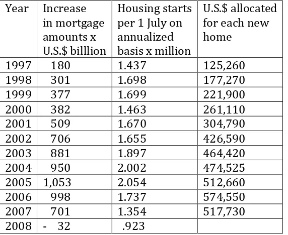
1997 has been chosen as the base year as in this year the increase in the mortgage amounts outstanding was $180 billion2_{, the new housing starts per 1 July of the same} year on an annualized basis were 1.437 million3_{, the median U.S. house price was} $145,900 in July 19974_{and the amount allocated to each individual new housing start} was $125,260. The latter amount was determined by dividing the increase in mortgage amounts outstanding by the new housing starts in the same year. The median U.S. house price rose to $149,900 in July 1998 and the amounts spend per new home rose to $177,270. 1998 was the turn around year.

Table 1 sets out the money input into the new housing starts and the average output price of the new homes for the period 1997-‐2008.

Table 1: Money input – new housing output and average money allocated per new home built over the period 1997-‐2008 in the U.S.

Year

Increase in mortgage amounts x U.S.$ billlion

Housing starts per 1 July on annualized basis x million

U.S.$ allocated for each new home

1997 180 1.437 125,260 1998 301 1.698 177,270 1999 377 1.699 221,900 2000 382 1.463 261,110 2001 509 1.670 304,790 2002 706 1.655 426,590 2003 881 1.897 464,420 2004 950 2.002 474,525 2005 1,053 2.054 512,660 2006 998 1.737 574,550 2007 701 1.354 517,730 2008 -‐ 32 .923

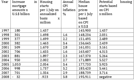
In table 2, in an alternative approach, the question has been answered how many new homes could have been started if U.S. home prices had increased in line with the Consumer Price Inflation Index (CPI).

1_{A Keynesian factor in monetary policy: the Economic Growth Incentive Method by Drs} Kees De Koning, 5th_{January 2015, http://mpra.ub.uni-‐muenchen.de/61129/}

2_{http://www.federalreserve.gov/releases/z1/current/accessible/b100.htm} 3_{https://www.census.gov/construction/pdf/bpsa.pdf}

[image:6.595.67.353.358.592.2]

(7)

Table 2: Potential Housing starts based on CPI basis

Year Increase in mortgage

amounts x U.S.$ billion

Housing starts

per 1 July on annualized basis x million

Annual CPI Inflation %

Median house prices per 1 July based on CPI x U.S.$

Potential housing starts based

on CPI x million

1997 180 1.437 145,900 1.437 1998 301 1.698 1.6 148,234 2.031 1999 377 1.699 2.2 151,495 2.489 2000 382 1.463 3.4 156,645 2.439 2001 509 1.670 2.8 161,031 3.161 2002 706 1.655 1.6 163,607 4.315 2003 881 1.897 2.3 167,370 5.264 2004 950 2.002 2.7 171,889 5.527 2005 1,053 2.054 3.4 177,733 5.925 2006 998 1.737 3.2 183,420 5.441 2007 701 1.354 2.9 188,739 3.714 2008 -‐ 32 .923 3.8 195,911 negative

Table 1 illustrates that the new money input into the housing market does not necessarily stimulate new homes being built. Over the period 1997-‐2005 money flows used by individual households to acquire homes show that higher and higher amounts of money were needed per each newly built home. Economic growth only occurs by building more homes and not by increasing the price of the total stock of homes far in excess of income developments.

Another way of expressing the development of the inefficient use of money in the home mortgage market in the U.S. over the period 1997-‐2007 is to calculate the Money Efficiency Index (MEI). This index is calculated by comparing the actual number of housing starts per annum with the potential number of housing starts. The latter was based on the CPI index plus the money input into the new housing starts. Table 3 provides the results.

Table 3 Money Efficiency Index

Year

Money

Efficiency Index

Year Money

Efficiency Index

1997 100 2003 36.0

1998 83.6 2004 36.2 1999 68.3 2005 34.7 2000 60.0 2006 31.9 2001 52.8 2007 36.5

[image:7.595.67.530.135.411.2] [image:7.595.67.503.636.771.2]

(8)

To understand the importance of this conclusion, one has to check the motives behind the borrowings. Population growth, changes in average family size and changing age and fashion patterns lead to a finite demand for new housing starts. Such demand is not based on supply levels, but on the need for shelter. When mortgages are on offer the restraining factor for an individual household is not the supply of homes, but the income level needed to support the loan facility. Individual households do not operate like companies; they do not seek to maximize profits as a home is for personal use. If capital gains are made, they are illusionary until the moment of sale. Rapid price rises for homes do undermine the efforts of the young to get on the property ladder.

In the U.S. the 42% gain in the number of new housing starts from 1997 to 2005 was totally offset by the 409% increase in the new money allocated per new home build. There has been an extremely low correlation between one extra dollar in home loans – the money input-‐ and the new housing starts –the economic output-‐.

Table 2 illustrates the same fact in a different manner. If house prices would have developed in line with the CPI inflation levels, the money allocated to new home starts would have made it possible to increase the level from 1.437 million in 1997 to 5.925 million in 2005. The U.S. did not need nearly 6 million homes to being built in 2005. Around 1.8 million would have been fully satisfactory. What is relevant in this context is that individual households’ income levels move much closer in line with the CPI levels than with the House Price Index.

Over the period 1997-‐2005 each new dollar borrowed for a home mortgage has had a rapidly declining impact on economic output and thereby economic growth. Table 3 illustrates the Money Efficiency Index, which clearly shows the increasingly inefficient use of money between 1998 and 2006.

The second consequence of the increasing inefficient use of funds has been that individual households joining the housing ladder had to allocate a larger and larger share of their incomes in order to be able to acquire a home. This reduces the freely available income for other consumption purposes.

These two factors: new money input into the housing market and an increasing debt service for new house buyers both lead to a reduction in economic growth rates.

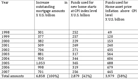
Another way to assess the impact of new mortgage lending volumes is to distinguish between funds used for new housing starts and funds used to increase the value of the housing stock over the CPI inflation level. Table 4 provides the details.

(9)

Table 4: Mortgage fund allocation over new home starts and changes in the housing stock valuation above the CPI inflation level over the period 1998-‐2007

Year Increase in outstanding

mortgage amounts X U.S. billion

Funds used for new home starts at CPI index level X U.S. billion

Funds used for Home asset price Inflation above CPI level

X U.S. billion

1998 301 252 49 1999 377 257 120 2000 382 229 153 2001 509 269 240 2002 706 271 435 2003 881 317 564 2004 950 344 606 2005 1,053 365 688 2006 998 319 679 2007 701 256 445

Total amounts 6,858 (100%) 2,879 (42%) 3,979 (58%)

Table 4 illustrates the growing importance of the funding element that does not contribute to economic growth: funds allocated to increase the housing stock values over and above the CPI inflation level. The 1998-‐2007 average percentage was 58%, but on an annual basis the peaks were reached in 2004 and 2006 at 68%.

Of each new mortgage granted over the period 1998-‐2007, on average 58% was used to increase house prices above CPI inflation levels. These borrowings burdened new mortgagees unnecessarily with excessive mortgage amounts.

The analysis of the above data may lead to the following conclusions:

1. The need for new homes is based upon population growth, changes in family size and changes in preferences for different types of homes. In the short term such need rarely changes rapidly. In the U.S. the need is for about 1.8 million new homes a year.

2. Home acquisitions are financed with own savings, often complemented with borrowed funds.

[image:9.595.67.527.204.466.2]

(10)

The evil force of borrowing and the weakness of Quantitative Easing©Drs Kees De Koning 3. The volume of newly borrowed funds for home acquisitions can have two very dissimilar effects: a volume effect on the number of new homes build and a price effect on the total housing stock. If, like in the U.S., the price effect starts dominating then new borrowings add less and less to economic growth while at the same time new mortgagees are burdened with mortgage levels that offer less value for money. Less value for money can be defined as the increase in the percentage of an income that has to be allocated for repaying the mortgage.

4. The individual households that suffer most from the declining values of income, are the new entrants to the housing market: the young and the lower income classes that have to borrow more percentage wise of their incomes than the more wealthy families.

5. When house prices start dropping, the households with the highest borrowing levels -‐ again the young and the new entrants to the mortgage market-‐ suffer the most. They suffer in two ways: firstly from the depreciation in home values and secondly from the loss in income earning opportunities through unemployment and wage increases below CPI inflation levels. Over the period 2006-‐2009 the values of households owner occupied real estate at market prices dropped by $5.57 trillion. During the period 1998-‐ 2007 the effects of overfunding the mortgage market by nearly $4 trillion led to a loss of about $5.6 trillion in home values in the three subsequent years. Between January 2008 and October 2009 7.8 million Americans lost their jobs. In 2013 the real median household income was 8% lower than the 2007 pre-‐recession level of $56,435. 5

2.2 Money input into the U.S. Federal Government and economic output

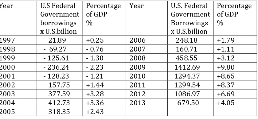
In table 5 the economic impact on GDP is measured from Federal government borrowings for the period 1997-‐2013.

Table 5: U.S. Federal government borrowings for the period 1997-‐20136

Year U.S Federal Government borrowings x U.S.billion

Percentage of GDP %

Year U.S. Federal Government Borrowings x U.S.billion

Percentage of GDP %

1997 21.89 +0.25 2006 248.18 +1.79 1998 -‐ 69.27 -‐ 0.76 2007 160.71 +1.11 1999 -‐ 125.61 -‐ 1.30 2008 458.55 +3.12 2000 -‐ 236.24 -‐ 2.23 2009 1412.69 +9.80 2001 -‐ 128.23 -‐ 1.21 2010 1294.37 +8.65 2002 157.75 +1.44 2011 1299.54 +8.37 2003 377.59 +3.28 2012 1086.97 +6.69 2004 412.73 +3.36 2013 679.50 +4.05 2005 318.35 +2.43

5_{http://research.stlouisfed.org/fred2/series/MEHOINUSA672N/} 6

[image:10.595.74.494.498.692.2]

(11)

The really remarkable changes in the U.S. government deficit funding over the period 1997-‐2013 was not that there was a surplus from 1998-‐2001, or a deficit due to military efforts in the Middle East from 2003, but the dramatic jump in deficit funding from 2009 onwards.

The total level of revenues for the U.S. Federal, States and local governments were $5.170 trillion in fiscal year 2007. This level of revenues dropped to $4.667 trillion in 2008 and a further drop to $3.665 trillion in 2009. No government can lower its expenditure level by just over $1.5 trillion or 29% in just two years; neither should it attempt to do so in the short run.

U.S. government expenses, including those funded by borrowed funds, lose their contribution to economic growth in the year after the expenditure has taken place. However the impact of borrowed funds will set back the disposable income growth for individual households for many years in the future. Hence the need for balanced budgets or for other solutions which help to get an economy back to its feet.

The experience of the U.S. shows that as a consequence of the individual households’ financial crisis brought about by years of neglect of the “money input -‐ new housing starts output relationship” U.S. government revenues dropped by 29% over the period 2007-‐2009. The real issue was and is that government revenues can be regarded as a lagging indicator of economic health. The leading issue was and is the financial health situation of individual households.

2.3 Some further conclusions

The relentless efforts to sell more and more mortgages during the years 1998-‐2007 were just like a car running out of control. Fannie Mae and Freddy Mac helped the banks to grow their mortgage business volumes rapidly. The extensive use of mortgage backed securities and credit default swaps made such business growth even easier. Banking supervision in the U.S. is a highly fragmented activity and shared between Federal and State agencies. No agency had over-‐all control over the mortgage market volumes. The free market philosophy, prevalent in the U.S. for many businesses, was seen as appropriate for all businesses including the financial sector.

Ever since 2008, the financial damage done to individual households, to the U.S. government at all levels and even to the banks should make economists rethink whether a mortgage volume growth objective should be given the overriding policy emphasis. How can such volume growth target be achieved? The U.S. banking system prefers to compete for business and is supervised by a fragmented banking supervision system. The losses inflicted on all sectors of business and the government, but last but not least on individual households do make it necessary to act in a manner that such irresponsible volume growth in mortgage lending does not occur again.

(12)

3 The choice between institutions and individual households

3.1 The adjustment process

The U.S. government, the Federal Reserve Bank and the individual households played the key roles in the adjustment process. Banks and the financial markets were rescued and companies adjusted their operations in line with expected demand levels.

3.1.1 The adjustment process for individual households

Contrary to many opinions, the adjustment period for individual households did not start in 2005 or 2006, but started already in 1998. In 1998 41.5% more money was used for each new built home compared to 1997 (See Table 1). Table 2 shows that 41.3% more homes could have been built if median house prices would have moved in line with CPI inflation. The potential number of new homes, which could have been built in 1998, would have been 200,000 more than required to meet annual long-‐term demand of 1.8 million new homes. This process of overfunding the housing market led to undermining the capacity to repay outstanding mortgages and also led to lowering the economic growth potential. This overfunding and undermining process continued to 2008.

When mortgage payment obligations can no longer be maintained, individual households find themselves in the unenviable situation to face the lenders. The statistics indicate that from the total housing stock in the U.S., 43.4 million homes are rented and individual households own 79.5 million homes. Of the 79.5 million homes owned, 49.2 million individual households have taken out a mortgage. The most shocking statistic is that over the period 2006-‐2013 22.1 million households in the U.S. did face foreclosure proceedings7_{and 5.8 million homes were repossessed. The 22.1 million constituted} more than one out of every 6 households in the U.S. The 5.8 million repossessed homes affected nearly one out of every 8-‐mortgage holder.

All that one can conclude out of this overfunding process is just how economically inefficient such mortgage funds have been used with the very sad results of dramatically increased unemployment levels, a wage level growth below CPI inflation levels for a number of years since 2008 and a priority allocation of households incomes to repaying outstanding mortgage debt at the detriment of buying other consumer goods and services. Over and above all this, during this process over the last 7 years, 5.8 million households lost all their savings in their homes. On top of this all, individual households reduced their collective home mortgage outstanding amount by $1.2 trillion from the end of 2008 to the end of the third quarter 20148_{; this represents an 11.4% drop in the} level of outstanding mortgage amounts.

7_{http://www.statisticbrain.com/home-‐foreclosure-‐statistics/}

(13)

As a consequence of this disastrous overfunding process and the subsequent efforts to get the outstanding amounts repaid, the U.S. government (Federal, State and local governments) saw their revenues flow drop by $2 trillion over the period 2007-‐2009. Over the period 2009-‐2013 U.S. government debt increased by at least $3.5 trillion more than could have been expected if the home funding crisis had not taken place. This economically inefficient use of funds for the home mortgage market led to a further inefficient use of funds for the individual households through the exacerbated deficit funding of the U.S. government. All in all the real victims of the inefficient home mortgage funding process were the individual households. They were the direct victims in lost income and spending opportunities, in reduced earnings, in increased unemployment levels and in an accelerated government debt level.

3.1.2 The adjustment process for the U.S. government

The U.S. government, like all other governments, has an ambition as to which services to provide to the general public. Priorities are decided by the Houses of Congress in the U.S. or parliaments elsewhere. There is often a fierce debate about which type of services should be included and which should be left to the private sector. The followers of John Maynard Keynes were of the opinion that government budgets were the appropriate tool to stimulate employment creation by incurring additional government deficit funding.

When outstanding government debt levels were around 30% of GDP, this would have made sense. However current government debt levels of many countries in the world, including the U.S., are at 80% of GDP or over. In the case of the U.S. government debt level (Federal, State and local) it is forecasted to reach $21.845 trillion for fiscal year 2015, well above the U.S. GDP level.

Tables 1-‐5 showed that the main increase in government deficit funding occurred as a consequence of the overfunding of the U.S. housing market and the subsequent efforts to claim back those funds from individual households. The U.S. government saw its revenues drop by 29% over the period 2007-‐2009. The deficit funding maintained government programs, but did and could not help individual households to get out of their debt position. A Keynesian solution of additional government debt creation on top of this all would have incurred major economic risks.

3.1.3 The adjustment process chosen by the Federal Reserve

The Federal Reserve's response to the financial crisis and actions to foster maximum

employment and price stability according to its own description.9

“The Federal Reserve responded aggressively to the financial crisis that emerged in the summer of 2007. The reduction in the target federal funds rate from 5-‐1/4 percent to

(14)

effectively zero was an extraordinarily rapid easing in the stance of monetary policy. In addition, the Federal Reserve implemented a number of programs designed to support the liquidity of financial institutions and foster improved conditions in financial markets. These programs led to significant changes to the Federal Reserve's balance sheet.

While many of the crisis-‐related programs have expired or been closed, the Federal Reserve continues to take actions to fulfill its statutory objectives for monetary policy: maximum employment and price stability. Over recent years, many of these actions have involved substantial purchases of longer-‐term securities aimed at putting downward pressure on longer-‐term interest rates and easing overall financial conditions.

The tools described in this section can be divided into three groups. The first set of tools, which are closely tied to the central bank's traditional role as the lender of last resort, involve the provision of short-‐term liquidity to banks and other depository institutions and other financial institutions. The traditional discount window, Term Auction Facility (TAF), Primary Dealer Credit Facility (PDCF), and Term Securities Lending Facility (TSLF) fall into this category. Because bank-‐funding markets are global in scope, the Federal Reserve also approved bilateral currency swap agreements with several foreign central banks. The swap arrangements assist these central banks in their provision of dollar liquidity to banks in their jurisdictions.

A second set of tools involves the provision of liquidity directly to borrowers and investors in key credit markets. The Commercial Paper Funding Facility (CPFF), Asset-‐ Backed Commercial Paper Money Market Mutual Fund Liquidity Facility (AMLF), Money Market Investor Funding Facility (MMIFF), and the Term Asset-‐Backed Securities Loan Facility (TALF) fall into this category.

As a third set of instruments, the Federal Reserve expanded its traditional tool of open market operations to support the functioning of credit markets, put downward pressure on longer-‐term interest rates, and help to make broader financial conditions more accommodative through the purchase of longer-‐term securities for the Federal Reserve's portfolio. For example, starting in September 2012, the FOMC decided to increase policy accommodation by purchasing agency-‐guaranteed mortgage-‐backed securities (MBS) at a pace of $40 billion per month in order to support a stronger economic recovery and to help ensure that inflation, over time, is at the rate most consistent with its dual mandate. In addition, starting in January 2013, the Federal Reserve began purchasing longer-‐term Treasury securities at a pace of $45 billion per month. In December 2013, the FOMC announced a modest reduction in the monthly pace of asset purchases and indicated it would likely reduce the pace of asset purchases in further measured steps at future meetings if incoming data pointed to continued improvement in labor market conditions and inflation moving back toward the Committee’s 2 percent longer-‐run objective.”

(15)

Some observations can be made about the Fed’s response.

1. The first one is about the start of the crisis. As tables 1 and 4 show the crisis of overfunding the mortgage market started in 1998 and not in 2007. In 2007 one could observe the collapse of the home mortgage debt mountain built up since 1998.

2. House price inflation, which affects all newcomers to the housing market, was not regarded as relevant to the inflation objective of 2%. Forcing individual households to spend a higher and higher percentage of their incomes on servicing mortgage debt has had a detrimental effect on overall economic growth levels.

3. New housing starts do not reflect general supply and demand theories, as demand is a finite rather than an unlimited one. The U.S. needs about 1.8 million new housing starts a year. In 1998 the increase in mortgage amounts outstanding would already have made it possible, if house prices had moved up in line with CPI inflation levels, to build 200,000 homes more than needed. Overfunding, rather than underfunding, was the main cause of the financial crisis, which started in 1998. Over the years’ 1998-‐2007 increasing money flows into the housing market created less and less economic growth. The Money Efficiency Index showed the extent of the inefficiencies as did table 4.

4. Banks (including Fannie Mae and Freddy Mac) competing for customers in making funds available to the home mortgage markets do not take into account the macro-‐ economic effects of overfunding a housing market with a finite need for new homes. Competition among banks does not lead to limits on the volume of funds lend.

5. The effectiveness of the interest rate as a tool to guide money to its best use should be called into question. The two main borrowing groups: a government and individual households do not behave like companies. For companies it is a cost among others to take into account when assessing profitable ventures. Companies also have a buffer in equity capital, which lowers the effectiveness of interest rate changes. Governments, generally speaking, take very little notice of interest rate changes as they assume that tax revenues will have to make up any shortfall; in other words the tax payers are the ultimate victims of any interest rate increase, while governments will easily find ways to spend tax revenues when interest rates drop. Why would it be sensible for a central bank to raise interest rates for slowing down house price inflation above the CPI level? There is a defined need for new homes and a defined need for borrowing levels. Both are not determined by markets but by population growth etc. If interest rates are increased to slow down lending for mortgages, such action will have undesirable consequences for both a government and companies. Neither of these two groups have anything to do with the lending volume for a single purpose: home acquisitions.

(16)

more out of their incomes to repay mortgages, thereby reducing economic growth levels.

7. The one group most affected by the overfunding process were the individual households in the U.S. Of course some of the lending institutions and financial market participants would have gone bankrupt if no liquidity and financial market support would have been given. This would have been catastrophic for the U.S. as well as for other countries. However one should not forget that the banks (including Fannie Mae and Freddy Mac) were the ones responsible for all the lending decisions in the first place. No borrower can borrow unless the lender decides so.

8. Last but not least one cannot deny that Quantitative Easing as an instrument of economic re-‐adjustment has worked very slowly. Buying up past government debt titles and outstanding mortgage backed securities has helped banks to earn more income; it also helped hedge funds and the wealthier individual households with appreciating bond and share prices. It has helped to lower interest rates to historically the lowest levels for over forty years. This has hurt savers, including those saving for a pension pot. It also did not induce home mortgage borrowers to borrow more, rather to the contrary. As stated, between 2008 and the end of the 3rdquarter 2014 borrowers reduced their outstanding by $1.2 trillion. The key element missing in quantitative easing was to consider the financial position of individual households, not in a very indirect manner but in a direct way. Individual households were not responsible for the increase in outstanding mortgage volumes, especially in respect to the volume of funds allocated to pushing house prices up faster than the CPI index and income growth of households. The collective of banks plus Fannie Mae and Freddy Mac were. If households had been helped in their liquidity position from as early as from 2008, the adjustment period would have been substantially shortened and economic growth rates would not have been dropped so drastically. The U.S. government would not have seen its revenues drop so severely. How the Economic Growth Incentive Method could have worked and still can work for European countries will be set out in the next section.

4. The Economic Growth Incentive Method (EGIM)

The readjustment period for the U.S. economy has taken well over 6 years from the start of 2008. As a result of the home mortgage market crisis in the run up to 2008, the whole economy was affected: companies, individual households and the Government’s finances. A finance-‐induced crisis needs a finance-‐induced answer.

The Federal Reserve did save the banks, apart from one. It did save the financial markets from collapse. It did lower short and long-‐term interest rates and it did monetize $2.461 trillion of government debt and $1.737 trillion in mortgage debt as per its balance sheet of 31 December 2014.10

The real question is: Would it have been possible to shorten the adjustment period?