NBER WORKING PAPER SERIES
THE PRACTICE AND PROSCRIPTION
OF AFFIRMATIVE ACTION IN HIGHER EDUCATION:
AN EQUILIBRIUM ANALYSIS
Dennis Epple
Richard Romano
Holger Sieg
Working Paper 9799
http://www.nber.org/papers/w9799
NATIONAL BUREAU OF ECONOMIC RESEARCH
1050 Massachusetts Avenue
Cambridge, MA 02138
June 2003
The authors thank Allan Meltzer, seminar participants at Carnegie Mellon University, Johns Hopkins University, Stanford University, and the University of Wisconsin for their comments and the National Science Foundation and MacArthur Foundation for financial support. The views expressed herein are those of the authors and not necessarily those of the National Bureau of Economic Research.
©2003 by Dennis Epple, Richard Romano, and Holger Sieg. All rights reserved. Short sections of text not to exceed two paragraphs, may be quoted without explicit permission provided that full credit including © notice, is given to the source.
The Practice and Proscription of Affirmative Action in Higher Education:
An Equilibrium Analysis
Dennis Epple, Richard Romano, and Holger Sieg
NBER Working Paper No. 9799
June 2003
JEL No. I20, I28, L3
ABSTRACT
The paper examines the practice of affirmative action and consequences of its proscription on the
admission and tuition policies of institutions of higher education in a general equilibrium. Colleges
are differentiated ex ante by endowments and compete for students that differ by race, household
income, and academic qualification. Colleges maximize a quality index that is increasing in mean
academic score of students, educational resources per student, an income-diversity measure, and a
racial-diversity measure. The pool of potential nonwhite students has distribution of income and
academic score with lower means than that of whites. In benchmark equilibrium, colleges may
condition admission and tuition on race. In a computational model calibrated using estimates from
related research, equilibrium has colleges offer tuition discounts and admission preference to
nonwhites to promote racial diversity. Equilibrium entails a quality hierarchy of colleges, so the
model predicts practices and characteristics of colleges along the hierarchy. Proscription of
affirmative action requires that admission and tuition policies are race blind. Colleges then use the
informational content about race in income and academic score in reformulating their optimal
policies. Admission and tuition policies are substantially modified in equilibrium of the
computational model, and both races are significantly affected. Representation of nonwhites falls
significantly in all colleges. The drop is particularly pronounced in the top third of the quality
hierarchy of colleges.
Dennis Epple
Richard Romano
Holger Sieg
Graduate School of
University of Florida
GSIA
Industrial Administration
[email protected]
Carnegie Mellon University
Carnegie Mellon University
5000 Forbes Avenue
Posner Hall, Room 233C
Pittsburgh, PA 15213-3890
Pittsburgh, PA 15213
and NBER
and NBER
[email protected]
The Practice and Proscription of Affirmative Action in Higher Education: An Equilibrium Analysis Dennis Epple, Richard Romano, Holger Sieg
I. Introduction
Consideration of race in admissions and provision of financial aid has become common practice among selective institutions of higher education, excepting instances where it has been banned.1 While college and university decision makers have shown a willingness to promote racial diversity with affirmative action policies, these practices are under legal and legislative attack. The University of California’s Board of Regents eliminated race- (and sex-) based affirmative action policies in 1995, this ban expanded to all public institutions in California by referendum in 1996. The state of Washington followed suit by passing an identical referendum in 1998. The Fifth Circuit Court of Appeals ruled against race-related admissions in Hopwood vs. Texas (1996), eliminating such practices in universities receiving public funding in Louisiana, Mississippi, and Texas. The use of race in admissions at the University of Georgia was proscribed by federal court in Johnson vs. University of Georgia (2001). At Governor Jeb Bush’s urging, the Florida legislature eliminated affirmative action at Florida public universities in 2000. As we write this paper, the U.S. Supreme Court is on the verge of ruling on affirmative action in higher education, having already heard arguments about the University of Michigan’s affirmative action policy.2
This paper develops an equilibrium model of the practice of affirmative action by colleges and analyzes the consequences of its proscription.3 In the model, colleges maximize a quality index that increases with academic qualification of the student body, inputs provided per student, and simple measures of racial and income diversity. Colleges are differentiated ex ante by access to nontuition revenues, which we refer to as endowment earnings. Potential students differ by race, income, and
academic qualification, and they maximize a utility function that increases in the quality of their education. We find a variant of a monopolistically competitive equilibrium, first allowing affirmative action practices. Equilibrium has a quality hierarchy of colleges, with an associated partition of the type space of potential
1
Evidence on the practice of affirmative action in higher education is discussed below.
2
Federal precedent at the time we write this is from the Supreme Court’s Bakke decision in 1978, a challenge to affirmative action in higher education under Title VI of the Civil Rights Act of 1964. The majority opinion by Justice Lewis Powell condemned quotas but ruled that admission officers could “take race into account” in admissions. This is discussed further below.
3
By “colleges” we mean providers of four-year college degrees, including the undergraduate divisions of universities.
students into colleges and a no-college alternative. For realistic parameterizations, colleges provide merit and need-based aid in equilibrium, and pursue affirmative action in admissions and provision of financial aid. We specify and calibrate a counterpart computational model and compute an equilibrium.
We then examine the consequences of proscription of affirmative action. We presume that preferences of college administrators and potential students are unchanged, but that college policies must be race blind. In equilibrium, colleges weigh the informational content of income and academic
qualification about race in formulating race-blind admission and tuition policies. Students with nonracial characteristics that are more likely to be associated with minorities are given some preference in admissions and provision of financial aid. In the calibrated model, colleges give some preference to students with high or moderately high incomes who also have relatively low scores on standardized college entrance exam, these students relatively more likely to be minorities. In spite of colleges’ strategies to maintain diversity, we find computationally that minorities are significantly hurt by proscription of affirmative action. For example, minority presence in the top tier of colleges declines by more than two-thirds. Non-minorities gain from elimination of affirmative action, but by very little with some exceptions.
Three strands of literature relate to this paper. The most closely related paper is by Chan and Eyster (forthcoming). They also analyze theoretically the proscription of affirmative action assuming, like us, that college administrators have preference for diversity and will employ alternative signals of race under the ban.4 They emphasize that such a ban may reduce the academic qualification of the admitted student body, when one motivation for such a ban is to improve academic credentials.5 Our analysis complements theirs, while differing in several important ways. Their model has one college, no
consideration of tuition, and no variation in incomes of potential students. With one college, their model abstracts from competition among colleges and there is no college quality hierarchy. Effects on access
4
See also Chan and Eyster (2002) which models the formation of preferences for affirmative action in college admissions, individuals taking into account the anticipated effects on their own admission prospects.
5
Loury, Fryer, and Yuret (2003) also investigate the consequences of a ban on affirmative action in a model where colleges maximize aggregate academic qualification of the student body subject to a racial quota and assuming the races have different costs of increasing their precollege academic qualifications. They also show that the ban will lower academic qualification of the student body given race-blind admissions that satisfy the racial quota. They go on to analyze the effects of the ban on costs expended to increase academic qualification. Our model of diversity preference does not employ a racial quota as discussed below. Otherwise, our analysis differs in very similar ways as from that of Chan and Eyster as discussed next in the text.
along the college quality hierarchy are a key element of our analysis. As well, we examine effects on tuition policies, and how this affects the races. Our inclusion of variation of income of potential students adds a realistic dimension to the analysis that is important to the nature of equilibria with and without affirmative action, and plays a key role in inference about race under the ban.
Second are our papers on higher education (Epple, Romano, and Sieg, 2002a & 2002b) and earlier papers with models of education that emphasize peer externalities (Rothschild and White, 1995, Epple and Romano, 1998 & 2002). Epple, Romano, and Sieg (2002b) develop and test a variant of the model of higher education employed here, but ignoring race issues. Epple, Romano, and Sieg (2002a) is a
preliminary analysis of introducing race preferences into the model, but with no analysis of proscription of affirmative action.
The third set of related papers are concerned with proscription of affirmative action either with no strategic response of colleges or as compared to some prescribed alternative. Kane (1998) estimates race-based preferences in college admissions and then shows that class-race-based affirmative action is a poor substitute. Kane (2000) provides evidence that high-school graduates ranking in the top 10 percent of their class and with lower than 80 percentile SAT scores are disproportionately minorities, suggesting an admissions strategy to enhance diversity at selective colleges. Long (2002a) also estimates preferences given to minorities in college admissions and then uses these estimates to forecast the effects of a ban on affirmative action with no substitute policy and also if a policy of admitting top-10 percent graduates from high schools is substituted.6 In Chapter 2 of their comprehensive analysis of affirmative action in a set of selective U.S. colleges, Bowen and Bok (1998) forecast effects on African Americans of banning affirmative action assuming probabilities of admission for a nonracial profile are as for whites. Cancian (1999) examines the substitutability of class-based for race-based admissions. The present paper is
differentiated from this line of research in our modeling of equilibrium provision of higher education with a set of competing colleges and our allowing colleges to respond strategically to a ban.
We close this Introduction with a brief discussion of evidence on affirmative action practices in higher education. These studies focus on admissions or financial aid. Bowen and Bok (1998) detail the practice of affirmative action in admissions of African Americans in five highly selective colleges. One
6
See also Long’s (2002b) forecasts of effects on applications of minorities to colleges from a ban on affirmative action.
finding they report is that the probability of admission in 1989 for white candidates with SAT score in the range 1200-1249 was 19 percent, while 60 percent for African American candidates. Kane (1998) uses data from the High School and Beyond survey and estimates admission probability in 1984 with Black and Hispanic as (separate) explanatory variables. He finds significant affirmative action in the top two quintiles of four-year colleges (ranked by mean SAT), most strongly in the top quintile. Using data from the National Education Logitudinal Study on 1992 high-school graduates, Kane (2000) reconfirms affirmative action in admissions in top quintile colleges. Long (2002a) estimates admission probabilities to four-year colleges using data from the National Education Longitudinal Survey. He finds significant affirmative action in admission for minorities in the early 90’s at both upper and lower tier colleges, but with stronger preference at upper tier colleges. In the basic regression, for example, he estimates that being African American increases the “likelihood of acceptance by the equivalent of a 254 point increase in SAT or a two-thirds of a point increase in GPA (p. 11).”
Manski and Wise (1983) found evidence of significant tuition discounting to nonwhite students. This has been reaffirmed in subsequent research by Kane and Spizman (1994) and Epple, Romano, and Sieg (forthcoming). Using Tobit estimates of financial aid in 1995-96, we estimate an increase in financial aid on the order of $1,500 for African American and Hispanic students in public schools, with higher (lower) aid in private colleges for African Americans (Hispanics).7
Section II of the paper presents the theoretical model. Section III develops results assuming affirmative action is allowed. Section IV shows how theoretical predictions change under a ban on affirmative action. Section V describes the computational model. Computational results are presented in Section VI. Further interpretation and discussion is contained in Section VI. Section VII concludes.
II. Theoretical Model
Here we present the theoretical model. The economy consists of colleges and potential students. A. Students. A potential student is characterized by three variables: race (r), household income (y), and score (s) on standardized college admissions test. We will frequently refer to potential students as just students, when it is clear by context whether they attend a college or not. We specify “race” to be
7
The coefficient estimates on the minority dummies are highly significant, but those on the interaction with private colleges are not significant.
dichotomous, white (w) or nonwhite (nw). Let denote the proportion of students of race r in the economy.
r
Γ , r {w,nw},∈
Household income is continuous with range [0,ymax]. While having in mind a household decision
about college, we refer to y as student income or just income henceforth. Score is continuous with range [smin,smax]. The joint density function of race r’s score and income is given by fr(s,y), assumed positive on S
/ (smin,smax) x (0,ymax). Normalize the economy’s student population to one, and let
denote the population density of (s,y). In our computational model below, we will use SAT to measure score.
w w nw nw
f (s, y)=Γ f (s, y) Γ f+ (s, y)
8
“Score” can, however, be given a more general interpretation as a one-dimensional measure of academic qualification that combines performance on standardized exam, pre-college grades, and any other quantifiable measures of academic capability.9
Student utility is an increasing and twice differentiable function of a numeraire x, college quality q, and score: U = U(x,q,s). The numeraire is given by x = y – p, where p denotes tuition if a college is attended. Determination of college quality is discussed below. If no college is attended, q = q0, the
educational quality of high school.10 A special case of the model assumes utility is increasing in educational achievement a, which is an increasing function of educational quality (q) and score: U = U(x,a(q,s)). The latter interpretation is used for some of the normative analysis in Section VI. Most of our analysis is positive, however. Implications regarding variables such as financial aid policies, admission policies, the college quality hierarchy and the allocation of students across the college quality hierarchy are the same regardless of the reasons why quality appears in the utility function. For predicting those
variables, quality may be preferred simply because households and their students gain utility from attending a higher-ranked school, or quality may be valued because it affects achievement. While most predictions from the analysis that follows do not depend on which of the interpretations is adopted, implications regarding achievement clearly depend on which of these reasons underlies the preference for quality, and
8
While not all potential students take a college admissions test in reality, we assume those that would be
admitted and attend a college do so, hence that students can anticipate their score. In our analysis it is then equivalent to assume every potential student actually takes the test.9
Kane (2000) finds that SAT and high-school rank are both significant in predicting admission and college GPA at top quintile colleges.
10
Hence, we assume the quality of the “outside option” is the same for everyone. This assumption might be relaxed, perhaps by making q0 a function of income and/or race.
some normative implications differ as well. As we proceed, we will identify implications that depend on an achievement interpretation. Note that we are assuming preferences are independent of race. We
considered some alternatives to this in Epple, Romano, and Sieg (2002a). Here differences across the races derive solely from differences in their distributions over (s,y).
We assume a positive income elasticity of demand for educational quality:
U q U x 0. x ∂ ∂ ∂ ∂ ∂ > ∂ (1)
We also assume a non-negative “ability” elasticity of this demand:
U q U x 0. s ∂ ∂ ∂ ∂ ∂ ≥ ∂ (2)
Taking as given college’s tuition and admission policies, students choose among their educational options to maximize utility.
B. Colleges. By “colleges” we mean institutions of higher education that grant four-year degrees, hence, including the undergraduate divisions of universities. There are n colleges, differentiated ex ante by their “endowment earnings,” Wi, i = 1,2,…,n. All nontuition earnings of a college make up Wi (i ranges from 1
to n unless indicated otherwise). We assume Wi ≠ Wj for all colleges i and j, and number the colleges so
that W1 < W2 < … < Wn.
Each college chooses tuition and admission policies and educational inputs to maximize a quality index.11 College quality is assumed to be an increasing, twice differentiable, and quasi-concave function of mean student score ( ), educational inputs per student (I), a measure of student income diversity (Dθ y), and a measure of racial diversity (DR): q q There is no doubt that colleges care about at least three of the four variables in our quality functions. Colleges clearly pursue students with higher scores; other things constant, they would like higher instructional expenditures per student (e.g., lower
faculty/student ratios), and they would like a racially diverse student body. What is the evidence for the fourth (income-diversity) component? Empirical analysis (e.g., Epple, Romano, Sieg, forthcoming)
y R
i= (θ ,I ,D ,D ).i i i i
11
Tuition to a student can itself, of course, induce or prohibit attendance, so our specification of a separate admission policy is for clarity and analytical convenience.
confirms the commonplace observation that colleges vary financial aid with income (i.e., provide need-based aid). One might hypothesize that this is simply price discrimination arising through exercise of market power by colleges. In our model, price discrimination by income does indeed emerge from the exercise of market power, but colleges do not have sufficient market power to pursue such price
discrimination to the extent required to yield the income-based pricing that we observe in the data (Epple, Romano, Sieg, 2002b). Thus, we introduce a concern for income diversity into the quality function as a means of accounting for the observed degree of pricing by income. Note that colleges’ use of the term "need-based aid" is consistent with a concern for income diversity, though such a spin might be used as a convenient rationalization regardless of the motive for income-based pricing.
The simple measure of income diversity we adopt is Dyi =µy µi,
y
where µ is the mean income in
the population, is the mean income of students in college i, and we are assuming as is
empirically relevant.
y i
µ µi>µ
12
Similarly, our racial diversity measure is
u u i i r r R i i D =Γ Γ , u i r
where is the
under-represented race in college i (meaning ), and Γ denotes the proportion of the under-represented race in college i. As consistent with the evidence with exception discussed below, assume that
= nw will emerge in equilibrium for all colleges, implying we can simplify notation by writing
u i r r r i Γ Γ ,for r r< = iu i u i r R nw i =Γi Γnw D .
The peer student-score measure ( ) in the quality index embodies an ability-related peer effect on educational quality that could operate through several channels. This could be due to students learning from one another in and outside of the classroom, enhanced competition among students for grades, student-body effects on hiring and motivation of teachers, and/or a variant of Spencian signaling.
i θ 13
12 If
µi<µy, then ∂q ∂Dy≤0, though this will not be relevant to any results.
13
There is a large, growing, and controversial literature on peer effects by social scientists. Here we mention just some of the empirical studies by economists that are most closely related to our model. Most of the literature on peer effects on educational success concern primary and secondary education. Early studies are Coleman (1966), Henderson, Mieszkowski and Sauvageau (1978), and Summers and Wolfe (1977). Manski (1993) details the several difficulties in empirically identifying peer effects. Evans, Oates, and Schwab (1992) find no peer effects in schools on teenage pregnancy or dropping-out once selection is taken into account. Robertson and Symons (1996), Zimmer and Toma (1997), Hoxby (2000), and Ding and Lehrer (2001) are more recent studies that find evidence of peer effects on educational success.
When maximizing quality, colleges observe student type (r,s,y) and take as given the maximum alternative utility the student can obtain.14 We now develop college i’s problem assuming affirmative action is allowed, and develop modifications when it is proscribed in Section IV. Let α
denote the admission policy of college i, indicating the proportion of type (r,s,y) in the population that the college admits. Utility taking implies college i believes it can attract any proportion of students to whom it provides their alternative utility, a belief that must be fulfilled in equilibrium. Letting
i(r,s, y) [0,1]∈ i
α ( )⋅
i
p (r, s, y)denote college i’s optimal price to student (r,s,y), the maximum alternative utility to college i is given by:
(3)
j 1,2,...,n; j i;α ( ) 0isan optimalchoicej
a
i 0 j
U (r,s, y) Max U(y, q ,s), Max U(y p ( ), q , s) .
= ≠ ⋅ > = − j ⋅
Alternative utility is the maximum of the no-college option and utility attainable at a college willing to admit the student. Let p (q ( ); r,s, y)v i ⋅ denote the reservation price for attending college i, defined by:
. (4)
v a
i i
U(y p , q ( ), s) U (r, s, y)− ⋅ ≡
Given college i’s belief that a student is willing to attend if offered his alternative utility, charging admitted students their reservation price will always be optimal (as this will loosen college i’s budget constraint). Note that this also implies U ( ) U ( )ai ⋅ = aj ⋅ for all colleges i and j.
Costs of college i are given by:
(5)
i i i i i
C(k , I ) F V(k ) k I ; V , V= + + ′ ′′>0,
letting ki denote the number of students attending. We assume “custodial costs” F + V that are independent
of quality-enhancing educational inputs, implying an efficient scale
i * k i i k ≡Arg min C(k , I ) ki
that is independent of Ii.
We can write college i’s optimization problem:
Turning to research on peer effects in higher education, Sacerdote (2001), Zimmerman (1999), and Winston and Zimmerman (forthcoming) find peer effects between roommates on grade point averages. Betts and Morrell (1999) find that high-school peer groups affect college grade point average. Arcidiacono and Nicholson (2000) find no peer effects among medical students. As noted above, Epple, Romano, and Sieg (2002b) estimate a variant of the present model and find support for its specification, including peer student scores in college quality.
14
nw θ ,I ,µ ,k ,Γi i i i i ,α (r,s,y)i nw nw i i y i i Max q(θ ,I ,µ µ ,Γ Γ ) (6.0) s.t. α (r,s, y) [0,1] (r,s, y);i ∈ ∀ (6.1) (6.2) v nw nw v w w i i S i i
[α (nw,s, y)p (q( );nw,s, y)Γ f (s, y) α (w,s, y)p (q( );w,s, y)Γ f (s, y)]dsdy W C(k , I ); ⋅ + ⋅ ≥
∫∫
+ i (6.3) nw nw w w i i i Sk =
∫∫
[α (nw,s, y)Γ f (s, y)+α (w,s, y)Γ f (s, y)]dsdy;nw nw w w
i i i
i S
1
θ s[α (nw,s, y)Γ f (s, y) α (w,s, y)Γ f (s, y)]dsdy; k =
∫∫
+ (6.4) nw nw w w i i i i S 1µ y[α (nw,s, y)Γ f (s, y) α (w,s, y)Γ f (s, y)]dsdy; k =
∫∫
+ (6.5) and nw nw nw i i i S 1 Γ α (nw,s, y)Γ f (s, y)dsdy k =∫∫
. (6.6)Constraint (6.2) is the college’s budget constraint, which embodies the optimality of charging admitted students (having αi>0) their reservation price.15
The budget constraint will hold with equality at the optimum since the objective function is increasing in educational inputs per student. Constraint (6.3) defines the number of students. Constraints (6.4) – (6.6) define, respectively, the mean score, mean income, and proportion of nonwhite students. In Section III, we present the solution to Problem (6). C. Equilibrium. Equilibrium satisfies utility maximization by students, quality maximization by the n colleges, and a market-clearance condition. Each potential student makes a utility-maximizing choice among colleges willing to admit the student (i.e., those for whom α is an optimal choice) and the no-college option, taking as given qualities and the admission and tuition policies of colleges. Each college solves Problem (6), taking as given its endowment and the alternative utility of potential students (or,
equivalently, the reservation price function). Market clearance requires that for all (r,s,y)
i(r,s, y) 0> n i 1=
∑
α (r,s, y) 1i ≤15
for an optimal αi( )⋅ for each college.16 If , then there would be excess demand by colleges
for students, and colleges would fail to optimize. If , then 1 of these students
can do no better than “choose” no college. The problem that colleges solve when affirmative action is proscribed changes, as then does the definition of equilibrium, as discussed in Section IV.
n i i 1 α (r,s, y) 1 = >
∑
n i i 1 α =∑
(r,s, y) 1< n i i 1 α (r,s, y) = −∑
i(r, s, y) ≡ i y) EM = > = < ; r,s, y), i s, y); = v i i 1 ,1] as p (q ; r,s, 0 ∈ nw i Γi nw i I (Γ 1); q − µ i I I (µ −y θ i i q q I (θ s) q q + − + nw i Γ nw i i I q Γ ; q + µ i I I q (µ q + q θ i i q I + (θ s)− I q 0; k R I = > − ∂ ∂III. Theoretical Results Allowing Affirmative Action
A. The College Optimum. College i’s optimum satisfies p p (qv budget balance (i.e., (6.2) with equality), the definitional conditions (6.3) – (6.6), and the following first-order conditions:
(7.1) α (r,s, y) [0 C (r, i q EMC (nw, s, y) V≡ ′+ )+ (7.2) i EMC (w,s, y) V≡ ′+ −y) (7.3) i i λ (7.4)
where (7.1) – (7.3) hold for all student types, is the multiplier on the budget constraint (6.1), and R denotes tuition revenues (i.e., the integral term in (6.2)).
i
λ
17
Condition (7.1) describes the admission policy, using what we call a student’s effective marginal cost of admission (EMC). EMC for nonwhites and whites are defined respectively in (7.2) and (7.3), these differing only by the last term. The first two terms in EMC equal the marginal resource cost of educating any student. The third term is the peer “ability” effect, equal to the change in mean score from attendance by a type s student, multiplied by the resource cost of maintaining quality. Note that this “cost” is negative for students with score exceeding the college’s mean
16
As shown below, any is optimal for some (r,s,y) for each college i in equilibrium. These student types are assumed to have access to college i when solving utility maximization, while market clearance is fulfilled using the actual number of students that exercise that option.
i
α ( ) [0,1]⋅ ∈ 17
score. The fourth term quantifies the analogous effect on the income-diversity measure. Note that since this cost is positive (negative) for students with income above (below) the college’s mean income. The last term is the cost of the effect on racial-diversity, which can again be analogously decomposed, but differs across the races. The cost of admitting a student from the under-represented race (nonwhite) is negative since while positive for the over-represented race.
i µ q < ,0 nw i Γ <1, 18 R I ∂ ∂
The economic implication of (7.4) is that college i spends more on educational inputs than the Samuelsonian level, as the latter would equate the collective marginal willingness to pay in the college (equal here to since students pay their reservation prices) to the marginal cost (k Colleges value educational inputs both for their revenue generating effect and for the direct effect on quality. In
equilibrium, colleges will be differentiated and have some market power, allowing them to depart from student optimality (i.e.,
i).
i
λ < ∞).19 It is of interest to note that profit-maximizing colleges would adopt the
same admission criteria, but would choose Samuelsonian levels of inputs.20
B. Properties of Equilibrium with Affirmative Action. Perhaps the most basic property of equilibrium is that a strict educational quality hierarchy characterizes equilibrium.
Proposition 1. qn>qn 1− >... q> 1>q0.
Proof of Proposition 1. All colleges solve the same problem (6) but with different endowments, implying the strict hierarchy that follows the endowment hierarchy among colleges. Using our assumption that Wn
< F, some students pay positive tuition at every college, implying q0 < q1. ,
While the college quality hierarchy follows the endowment hierarchy, a strict hierarchy would need to characterize equilibrium if colleges had the same endowments. The hierarchy with the same endowments is driven by preferences of higher-income types for higher-educational quality and can be proved following an argument like that developed in Epple and Romano (1998,2002).21
To establish some of the results that follow, it is convenient to let EMC0(r,s,y) 0 denote the
hypothetical effective marginal cost of the no-college option. We appeal to the panels of Figure 1 from our
≡
18
In our model, affirmative action is quite different from a racial quota as discussed in Section VII.
19
Students would prefer that colleges provide Samuelsonian levels of inputs and lower tuition.
20
This is shown by solving a college’s profit-maximization problem. Epple and Romano (1998,2002) develop equilibria in a related environment with profit maximizers.
21
computational analysis to illustrate some of the results. The solid lines in Figure 1 show the partition by race of the (s,y) plane into colleges and the no-college alternative in computed equilibrium. The functions and parameters that underlie this example are discussed in Section V.
Another fundamental property of equilibrium is non-overlapping attendance sets for given race. Proposition 2. Given r, the set of (s,y) types that attend college i and college (or no college if j = 0) is of measure 0.
j i≠
Proof of Proposition 2. Given r, if type (s,y) attends i or j in equilibrium (i,j = 0,1,…,n; i ), then If either equals 1, then market clearance would be violated. From (7.1), tuition at college i and college j then equals EMC there. (If say j = 0, then use the convention that EMC
j ≠ i j α ∈(0,1) andα ∈(0,1). α or αi j j 0 =
0.) Using utility maximization, it must then be that
(8)
i i j
U(y EMC (r,s, y), q ,s) U(y EMC (r, s, y), q ,s)− = −
for these types. If, say, utility were higher at option j than at option i, then the reservation price for attending college j would exceed EMCj (a contradiction to optimal pricing); or if j is the no-college option,
none of these types would attend i. Given qi ≠qjby Proposition 1, EMC (r, s, y) EMC (r,s, y),i ≠ j implying
ds dygiven (8) is satisfied is generically unique in the parameter space of utility functions U( ).⋅ ,
For given race, we refer to the loci in the (s,y) plane that partition student types into colleges and no college as boundary loci. These loci are equations (8) where i and j are the best options of these types and students on one side choose option i and those on the other choose option j. The panels of Figure 1 provide an example with n = 5 (developed in detail below), where the solid lines are boundary loci. In each panel, the lower left “triangle” of types do not attend college, and the diagonal slices are the attendance sets at progressively higher quality colleges.
Proposition 3 concerns tuition policies:
Proposition 3. a. Along a boundary locus of college i, p (r, s, y) EMC (r,s, y).i = i
b. In the interior of college i’s attendance set (i.e., off boundary loci), p (r, s, y) EMC (r,s, y).i > i
c. Equilibrium student choices are the same as would result if p (r, s, y) EMC (r,s, y),i = i i = 1,2,…,n, for all
(9)
j 0,1,...,n; j i
i i j j
U(y EMC ( ), q ,s) Max U(y EMC ( ), q ,s),
= ≠
− ⋅ ≥ − ⋅
with strict inequality in the interior of attendance sets.
Proof of Proposition 3. a. This follows from the definition of boundary loci and the Proof of Proposition 2. b. Tuition pi < EMCi to a student attending college i contradicts (7.1). Tuition pi = EMCi in the interior of
college i’s attendance set and pj = EMCj at the best alternative j would contradict Proposition 2. Tuition pi
= EMCi and pj > EMCj at the best alternative j would contradict market clearance (since then α
Tuition p
j=1).
i = EMCi and pj < EMCj at the best alternative j is impossible, since pj < EMCj implies j is not an
option for the student.
c. Contradicting (9), suppose that a student attends option i, when
for some Since p
j j i i
U(y EMC , q ,s) U(y EMC , q ,s)− > −
j j i i
U(y EMC , q ,s) U(y p , q ,s).− > −
i j α α+ >1). , j i.≠ EM ⋅ > i EMC≥ ying i by (7.1) (and by definition if i = 0),
If j = 0, then utility maximization would be contradicted. If j ≠ 0, then
and thus that market clearance is violated (as then Having established (9), the alternative to it holding with strict inequality in the interior of an attendance set would have it hold with equality (at least for some values of (r,s,y)). This would contradict Proposition 2.
v
j j
p (q ; ) C ,impl α 1j=
The results in Proposition 3 are quite intuitive. On boundary loci, students are indifferent to the adjacent options with tuitions equal to EMC, implying higher tuition would drive away the students. Since EMC declines with score and increases with income in any college, merit aid and need-based aid are implied along boundary loci. Likewise, financial aid is provided to the under-represented race. Moving into the interior of attendance sets, preferences change so that students would have strict preference for the college attended if EMC-pricing prevailed. The attended college then increases tuition, taking away the consumer surplus that would otherwise result. Reference to the panels of Figure 1 provides further clarification. Consider the students who attend the lowest quality college in equilibrium, those lying between the bottom two lower-left boundary loci (solid curves) in each panel. Those on the bottom boundary loci are indifferent to the no-college option, their best alternative to college 1, and face tuition equal to EMC1(Α) at college 1. Moving above the bottom boundary locus slightly, these students continue
them indifferent to no college. This is so until the dashed line between the bottom two boundary loci is reached (which is only slightly above the bottom boundary locus in Figure 1), this dashed locus equation (8) with i = 0 and j = 2. Crossing this locus, students have college 2 as their best alternative with access at p2 = EMC2, and this option dictates tuition at college 1. Similarly, those who attend college 2 have either
college 1 or college 3 as their best alternative, as delineated by the dashed curve, and so on.22
The price discrimination in the interior of attendance sets is not very pronounced for realistic parameterizations (as below), implying merit aid, need-based aid, and discounting to the under-represented race prevails.23,24 Since it is in the interest of any college to attract any student willing to pay more than EMC, the price discrimination that is practiced will not disrupt the allocation implied by EMC-pricing (i.e., Proposition 3c), a variant of a standard result concerning first-degree price discrimination.
Proposition 4 summarizes the effects of the preference afforded to members of the under-represented race who attend college in equilibrium.
Proposition 4. a. Higher Utility. Members of the under-represented race who attend college have higher utility than those from the other race with the same (s,y), with the exception of those from the under-represented race with no college as their best alternative (who have the same utility as their counterparts from the other race).
b. Lower Tuition. Members of the under-represented race with the same (s,y) and in the same college as members of the other race pay lower tuition, with the exception of those from the under-represented race who have no-college option as their best alternative (who pay the same tuition as their counterparts from the other race).
c. Higher College Quality. If the shadow value of racial diversity rises along the college quality hierarchy (i.e., if (q increases with i), then, for given (s,y), the quality of education is at least as high for the
under-represented race. nw i I i Γ / q )
22
Boundary loci might meet (but cannot cross), in which case the partition is somewhat more complicated but tractable. See Epple and Romano (2002) for related examples.
23
One can derive further results about properties of pricing for particular specifications of utility, including the Cobb-Douglas specification adopted in our computational model below.
24
The top college exercises “more” price discrimination since it faces competition only on the lower side of the quality hierarchy.
Proof of Proposition 4. a. We show first that, if a student (r,s,y) attends college i in equilibrium, then v i i p ( ) p (q , )⋅ = ⋅ satisfies: (10) j 1,2,...,n; j i i i j j
U(y p ( ), q ,s) Max U(y EMC ( ), q , s).
= ≠
− ⋅ = − ⋅
Since α ( ) 0i ⋅ > in equilibrium, market clearance implies p ( ) EMC ( )j ⋅ ≤ j ⋅ for all j≠i. If p ( )i ⋅ exceeds the
value satisfying (10), then p (q ; ) EMC ( )v j ⋅ > j ⋅ for some college j i, a contradiction (or the no college
option is preferred to i, also a contradiction). If p
≠
i(⋅) is below the value satisfying (10), then, since
j j
p ( )⋅ ≤ EMC (⋅) for all j ≠i, p ( ) p (q ; ),i ⋅ < v i ⋅ a contradiction to quality maximization by college i. This
establishes (10). The result then follows since EMCj(nw,s,y) < EMCj(w,s,y) for all j 0 and
EMC
≠
0(nw,s,y) = EMC0(w,s,y).
b. This follows as well from the proof of part a of this proposition. c. Suppose the alternative, which by Proposition 3c implies:
(11)
i i j j
U(y EMC (r,s, y), q , s) ( ) U(y EMC (r,s, y), q ,s) for r w (nw),− ≥ ≤ − =
for some (s,y) and colleges i and j having qi > qj. To simplify notation here, let nw i i Γ z ≡(q q )I i j j i denote the
shadow value of racial diversity. Given the first inequality in (11),
(12)
i j i j j
j j
U(y EMC (w,s, y) z , q ,s) U(y EMC (w,s, y) z , q ,s) U(y EMC (nw,s, y), q ,s),
− + > − +
= −
the inequality in (12) by normality of demand for quality (see (1)) and the equality by definition (see (7.2) and (7.3)). By supposition, zi – zj > 0, this with (12) implying:
(13)
i i i j
U(y EMC (w,s, y) z , q ,s) U(y EMC (nw,s, y), q ,s).− + > −
Since the left-hand side of (13) equals (again by (7.2) and (7.3)), we have a contradiction of the second inequality in (11), implying the result. ,
i
U(y EMC (nw,s, y), q , s)−
The reason members of the under-represented race who attend college and have no college as their best alternative are not better off than their counterparts from the other race is that colleges price away surplus and utilities are the same across the races in the no-college alternative. Proposition 4c provides a sufficient condition, satisfied in our computational analysis, such that gains to the under-represented race
entail weakly higher quality education. While the condition is not necessary for this result in general, absent it a nonwhite might choose to attend a lower-quality college than a counterpart white, utility gains due to a substantial tuition break. It is important to keep in mind that the relatively more favorable outcomes for nonwhites we find in equilibrium depend on the “lower” distribution of (s,y) associated with nonwhites. In our model, if fw(s,y) / fnw(s,y), then outcomes are race neutral. While some nonwhites with
the same (s,y) as whites are better off due to affirmative action for realistic parameter values, nonwhite presence in colleges will be proportionally lower than for whites, so we do not mean to imply nonwhites are better off as a group.
As in the example in Figure 1, equilibrium will frequently exhibit within race income and score
stratification. By income stratification, we mean that, for given race and score, whenever a potential
student changes options as income rises, a higher-educational alternative is chosen. Income stratification will result as a consequence of normality of demand for educational quality, unless preference for income diversity causes sufficiently rising aversion to higher-income students by colleges as one moves up the quality hierarchy.25 We find that the shadow value of income diversity does rise at the top of the college quality hierarchy in our computational model below, but not by enough to disrupt income stratification. Score stratification for given race and income is defined analogously. A sufficient condition for score stratification is a weakly increasing shadow value of scores along the quality hierarchy.26 This
characterizes the equilibrium computed below (and numerous related specifications that we have analyzed). Note that the combination of income and score stratification for each race produces the “diaganolized” partition into colleges in the panels of Figure 1.
We do not have a proof of existence of equilibrium. We can show existence of an allocation that satisfies utility maximization, market clearance, and has all colleges at a local maximum of Problem (6). The difficulty in confirming that the allocation is an equilibrium is that the quality maximization problem is not a quasi-concave programming problem, so conditions for global optimality cannot be shown using standard methods. While we cannot then be certain that we compute equilibria below, because colleges are
25
For the specification of utility adopted in our computational model, there is a simple condition for income stratification. See footnote 30.
26
The shadow value of score in college i is the negative of the coefficient on s in EMCi (see (7.2)
and (7.3)).
θ I
at local optima (and the remaining equilibrium conditions are satisfied), the allocation is at least an equilibrium if we presume adjustment costs. Suppose that colleges bear adjustment costs:
w nw
S
K(
∫∫
[δ(w,s, y)f (s, y) δ(nw,s, y) f+ (s, y)]dsdy), with where δ isany deviation from the equilibrium admission policy α . Then for K” sufficiently high, the allocation we compute is an “equilibrium with adjustment costs.” For expositional ease, when we discuss the computed allocation below, we refer to it as just an “equilibrium.”
K(0) K (0) 0 and K= ′ = >0; y) ′′ i (r,s, y) (r,s,
IV. Theoretical Analysis with Proscription of Affirmative Action
We model the proscription of affirmative action practices by colleges as requiring that college policies are race blind. A college’s admission and tuition policies are then restricted to be functions of (s,y) only. Colleges will factor the informational content of (s,y) about race into their decision calculus in an effort to promote racial diversity.
Equilibrium is defined analogously. Colleges continue to maximize the same quality index, solving the modified problem presented below. The market clearance condition is here race blind:
with continuing to denote college i’s admission policy. Generally,
we will continue to use the same notation, but imposing the race-blind restriction on the functional arguments.
n i i 1
α (s, y) 1for optimalα (s, y),
=
≤
∑
α ( )⋅iA. Modified College Problem and Solution. Since the races are treated the same, the reservation price function is also race blind: pv = pv(qi;s,y). College i now solves:
nw θ ,I ,k ,µ ,Γi i i i i ,α (s,y)i nw nw i i y i i Max q(θ ,I ,µ µ ,Γ Γ ) (14.0) s.t. α (s, y) [0,1] (s, y);i ∈ ∀ (14.1) (14.2) v i i S
p (q( );s, y)α (s, y)f (s, y)dsdy W C(k ,I );⋅ +
∫∫
≥ i i(14.3)
i i
S
i i i S 1 θ sα (s, y)f (s, y)dsdy; k =
∫∫
(14.4) i i i S 1 µ yα (s, y)f (s, y)dsdy; k =∫∫
(14.5) and inw i nw nw i S 1 Γ α (s, y)Γ f (s, y)dsdy k =∫∫
. i (14.6)The solution has the same condition (7.4) describing choice of inputs (Ii), and race-blind
admission policy: (15.1) v i i 1 α (s, y) [0,1] as p (q ;s, y) EMC (s, y); 0 = > ∈ = = < i nw i µ θ i i i I I nw nw Γ nw i I q q EMC (s, y) V I (θ s) (µ y) q q q Γ f (s, y) Γ . q f (s, y) ′ = + + − + − + − i (15.2)
The race-blind EMC is analogous to that above (see (7.2) and (7.3)), except for the last term. With and without affirmative action, the last term in EMC measures the cost of admitting a student type on racial diversity, but now using (s,y) as a signal of race. Multiplying the term in parentheses at the end of (15.2) by 1/ki, one has the expected change in the diversity measure from increasing which is
then multiplied by the dollar cost of maintaining quality (
nw i Γ α (s, y)f (s, y),i nw i Γ I q q i
k ). Admitting types (s,y) with proportion
of nonwhites in the population of potential students exceeding the college’s proportion of nonwhites ( ) improves racial diversity, with then negative diversity cost. The diversity cost is, of course, positive (or zero) for the remaining set of student types.
nw nw nw
i
Γ f / f>Γ
B. Equilibrium Properties. The strict-quality-hierarchy property (Proposition 1) continues to characterize equilibrium with the same proof. Again, attendance sets do not overlap in the (s,y) plane, here for the races combined.27 As well, the properties of pricing and the allocation collected in Proposition 3 have
27
straightforward race-blind counterparts, and are shown by analogous arguments. Obviously, nothing akin to Proposition 4 regarding racial differences for given (s,y) holds here. Score and income stratification are more easily violated here due to using (s,y) type as a signal of race, although income stratification
continues to characterize the computations below. The existence issue is the same.
Predicting the effects of proscription of affirmative action on the provision of higher education, consumption of it by the races, and on normative measures depends on the functional and parametric properties of the environment. Hence, we turn to our computational specification.
V. Computational Model
To provide evidence regarding the quantitative effects of a ban on affirmative action, we employ a computational counterpart to our theoretical model. We generalize and refine the computational model in Epple, Romano, and Sieg (2002a). We use the shorthand ERS to refer to that source in the discussion that follows. In calibrating the model, we seek to characterize the distributions of income and test scores by race for the U.S. population. In doing so, we employ data from the U.S. Census, data purchased from Petersons that is a survey of the universe of colleges and universities, data from the NSF WebCASPAR system, and data on a sample of college students from the National Postsecondary Student Aid Survey of the National Center for Education Statistics (NCES). In addition, we use parameter estimates from our econometric analysis in Epple, Romano, and Sieg (forthcoming). The calibration is in 1995 dollars. The computational model has five “colleges” in addition to the non-college option.
The model has two races, whites and nonwhites. Data for nonwhites are obtained by combining data for African American and Hispanic students and households. We set the proportion of nonwhite potential students to .20, using 2000 Census data. The income distribution of each race is taken to be lognormal. In ERS, the parameters of the income distribution for each race are chosen to match mean and median incomes in the U.S. population. Here we modify the calibration so that average income of college attendees in the computed equilibrium equals the average income in the NCES data. The ratio of the mean incomes of nonwhites relative to whites is as in ERS and the standard deviations of the logarithms of income by race are from ERS. This yields ln(y) ~ N(9.92, .764) and ln(y) ~ N(9.85,.746) for whites and nonwhites respectively.
As with the distributions of income, the race-conditioned distributions of score are for the populations of potential students. The distributions thus characterize the scores of college attendees as well as predicted scores of those who do not attend college. The parameters of the distributions of score in the model are chosen so that the means and variances of ln(s) conditional on college attendance in computed equilibrium equal the means and variances of total SAT (in thousands) for white and nonwhite colleges attendees in the NCES data. This yields ln(s) ~ N(.924,.190) and ln(s) ~ N(.735,.20) for whites and
nonwhites respectively. The correlation of ln(y) and ln(s) for each race is set equal to the correlation for the population of students in the NCES data, yielding a correlation of .25. This completes the calibration of the joint distribution of income and score for the two races.
Endowments per student were chosen to correspond to those in the NSF WebCASPAR data. Colleges were ranked by SAT score and combined into five groups with an equal number of students in each group. Endowment per student was then calculated for each group. We assume that a draw of 2% per year from endowment is allocated to undergraduate education.28 This yielded endowment income per student of $155, $243, $386, $755, and $4149 for the five colleges.
The combined utility and quality function is chosen to be Cobb Douglas:
The parameters are thus the exponents on own score, inputs, mean score, income diversity, and racial diversity. We choose these parameters and the quality of the outside option so that the equilibrium level with affirmative action of college attendance of the two races combined corresponds to that observed in four-year colleges in the U.S. (estimated in ERS to be 28.2%) and equilibrium average cost per student approximately equals average instructional
expenditures reported in the NSF WebCASPAR data. The parameters of the utility-quality function are also chosen so that equilibrium shadow prices on income, score, and race correspond roughly to magnitudes we obtained from Tobit regressions of financial aid on those variables using the NCES data (Epple, Romano, and Sieg forthcoming). Those estimates were an approximate $1,100 increase in financial aid per standard deviation of SAT, $30 dollar reduction in aid per $1,000 increase in family income, and financial aid to
3 5 1 2 φ 4 φ φ φ y φ R U (y p) q s ; q I= − ⋅ ⋅ = θ (D ) (D ) ; ln(s) SAT.=
28
This is a somewhat arbitrary allocation since we do not have data with respect to the allocation of endowment funds across undergraduate, graduate, and research activities.
nonwhites relative to whites of $1,500. The exponents on inputs, mean score, income diversity, and racial diversity in the quality function are .0705, .0825, .02, and .0029 respectively.29
The custodial cost function (V(k) + F) was chosen to be cubic. Parameters were chosen to generate colleges that are roughly equal in size and to yield average custodial costs that are approximately one fourth as large as instructional expenditures per student. The cost function is: 33.43+200k+2,043k2 +925,000(k-k*)3+ Ik. Cost-minimizing scale in the chosen function is k*=.069.
Comparison of the equilibrium when affirmative action is permitted to the data is provided in Table 1, with the data based on the five college groupings described earlier. Income, SAT, and racial composition data are from the NCES. Inputs are instructional expenditures from NSF WebCASPAR. As the table reveals, input expenditures and SAT scores match reasonably well between the model and the data. Average SAT and average percent nonwhite also match reasonably well between the model and the data. In the data, minorities are not under-represented in the bottom tier of colleges, while our model predicts under-representation in all colleges. Average income from the model closely matches average income in the data, reflecting our calibration strategy, but the model predicts more income stratification than is present in the data. In our calibration, we did not impose a match between the model and data of the percent of college attendees who are nonwhite. Thus, it is encouraging to see that the equilibrium
percentage of college attendees that are nonwhite from the model (14.6%) is only slightly below the average in the data (15.3%). However, as is evident from the table, the model predicts a more equal distribution of nonwhites across colleges than is found in the data. Overall, given the parsimony of our model, we view the match between the model and data as encouraging.
VI. Computational Results
The top panel of Table 2 provides further detail regarding the equilibrium when affirmative action is permitted. Nonwhites are under-represented in each college. Note that the shadow prices on racial diversity ascend in the equilibrium. From part (c) of Proposition 4 it then follows that the quality of education for nonwhites is at least as high as for whites for given (s,y). This in turn is illustrated by a
29
The value of φ is irrelevant to the equilibrium allocations, and then need not be calibrated to compute equilibria with and without affirmative action. However, the value of φ is relevant to some of the normative analysis we pursue, and its calibration is discussed below.
1
comparison of the boundary loci for whites and nonwhites in Figures 1 and 2. The boundary loci are overlaid in Figure 2 to facilitate comparison of the admission spaces. The lower boundary loci for nonwhites relative to whites illustrate the improved access by nonwhites to quality colleges as a result of affirmative action. A comparison of average SAT scores and average incomes across colleges in the upper panel of Table 2 provides further illustration.30
Table 2 also reports shadow prices (sp) for score, income, and race, i.e., the coefficients on these variables in EMC (recall (7.2) and (7.3)). These shadow prices correspond closely to actual variation in tuition with student characteristics in colleges 1 through 4 in computed equilibrium.31 Those colleges thus have little market power, with tuitions closely approximating effective marginal costs. In college 5, the marginal increase in tuition with income is approximately twice as large as the shadow price. The marginal decrease in tuition with score is approximately half the shadow price on score and the discount to
nonwhites is approximately half the shadow price on racial diversity. These features of pricing in college 5 reflect the greater market power of the top college as compared to the remaining colleges, as it faces competition only from lower-quality colleges.
The bottom panel of Table 2 reports the equilibrium outcomes when affirmative action is
proscribed. This change results in a 35% drop in college attendance by nonwhites. This drop is particularly pronounced in the higher-ranked colleges and is accompanied by a dramatic increase in the shadow price on racial diversity along the quality hierarchy. In the top college, the attendance by nonwhites drops by two thirds. Recall that in our computational model, the top “college” represents the top tier of institutions. In the computed equilibrium the top college is attended by approximately 13.5% of the student population. Thus, a drop by two thirds in attendance of nonwhites in that set of institutions would be a very large impact. We should emphasize that our computational model is a Spartan representation of reality, and this should be kept in mind in thinking about the numerical estimates of the impact of proscribing affirmative action. However, the computational analysis supports the conclusion that the effects of proscribing affirmative
30
Income stratification results in this specification if quality multiplied by one plus the shadow value of income increases along the college quality hierarchy. This condition is satisfied here.
31
We investigated properties of tuition functions by generating a random sample of students from the distribution of types. We determined the school each student would attend in equilibrium and the tuition in that school. We then estimated linear regressions of tuition on income, score, and race for each college. All coefficients in these regressions were highly significant, and all the regressions have R2 values greater than .99. The text summarizes findings from these regressions.
action will be substantial and will be increasingly pronounced as one moves up the college quality hierarchy.
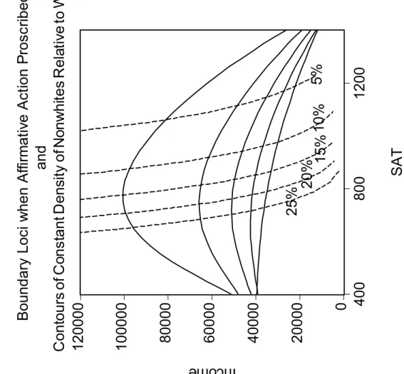
Admission spaces with and without affirmative action are shown by race in Figure 3. The solid lines are the boundary loci when affirmative action is permitted. The dashed lines, common to both races, delineate admission spaces when affirmative action is proscribed. Where the loci are shifted upward by a ban on affirmative action, college access is more restricted and conversely where the loci have shifted downward. A combination of three effects on effective marginal cost of admission of type (s,y) from proscribing affirmative action explains the changes in the admission spaces in Figure 3. Without affirmative action, (s,y) types with higher ratio of nonwhites in the population than in the college have lower EMC and are then relatively preferred by the college (recall the last term in parentheses in (15.2)). Figure 4 shows the boundary loci under the ban and introduces contours with constant ratios of nonwhites. Admission of relatively higher-income and higher-score types will worsen diversity, and the reverse for relatively lower-income and lower-score types. As seen in Figure 3, colleges modify their admission policies as they accept lower-scoring types with high and moderately high income, students who are relatively likely to be nonwhite, leading to the hump-shaped boundary loci without affirmative action. The second effect is that, relative to when affirmative action is permitted, the signal of race is weakened under the ban, this increasing EMC under affirmative action for nonwhites and decreasing it for whites. Mathematically, this corresponds to the increase in the term in parentheses in (15.2) relative to the counterpart term in (7.2) for nonwhites, and the reverse for whites (here comparing to (7.3)). This signal weakening corresponds to the loss in power to discount tuition to nonwhites and charge a premium to whites. The third effect is the change in the shadow value of racial diversity, which rises in equilibrium under the ban in all colleges. The three effects approximately offset at high scores for whites, which implies higher EMC for the same (s,y) for nonwhites due to the second effect. For high scores, boundary loci are approximately the same for whites but shift out for nonwhites. For whites, a ban on affirmative action improves college access particularly for those with relatively lower incomes and scores. For nonwhites, the shift is generally toward more restricted access except for those with relatively lower incomes and scores.
The upward sloping segment of the boundary loci under the ban raises the issue of incentive compatibility since some students have the opportunity to under perform on the exam and gain access to a higher quality college. The equilibrium allocation is, however, incentive compatible with respect to claiming a lower s than the actual value. Here we provide an intuitive explanation with proof in an appendix (available on request). In the equilibrium, we have verified that tuition declines with s in each college for given y. Hence, no student who would stay in the same college with a lower score would claim to have such an s. Neither would a student who would attend a higher quality college with a lower score underreport s. Utility of a student reporting a lower s while staying within any college declines as we have discussed, and utility of a student reporting an s that places him on a boundary locus is the same in each college (as is easily shown). Combining the latter facts implies incentive compatibility.
A comparison of the two panels in Table 2 reveals a rise in average SAT scores of nonwhites in lower-ranked colleges and a fall in higher-ranked colleges. This is a consequence of the reduced access of nonwhite students to higher-ranked colleges. We also see a higher average income for nonwhites relative to whites in colleges. To understand this phenomenon, first note that along the downward sloping portion of boundary loci (where most students fall), tuition declines as score rises, hence the minimum income level for admission also declines with score. This coupled with relatively more whites having higher scores induces lower average incomes of whites in colleges.
We calculate two normative measures on potential student types of the effects of proscribing affirmative action. One is the standard compensating variation of the ban. We also calculate the effect on educational achievement, using the interpretation of the utility function: U = U(y-p,a(q,s)). Reasons to examine separately effects on achievement are as follows. Social externalities from educational
achievement may be present that would have no effect on compensating variation. Role models provided by highly educated individuals are one potential example. The compensating variation measure is also suspect because the utility function may better be interpreted as a reduced form, suitable for describing behavior but not for standard normative analysis. We have required normality of demand for educational quality, consistent with observed behavior, but frequently interpreted as a manifestation of borrowing constraints. Last, because we are studying education, effects on achievement are also intrinsically of interest. While our results with respect to achievement rely on the assumption that quality affects utility via
its effect on achievement, we emphasize that this assumption is not required for any of our other computational results.
We first investigate the effects of affirmative action on achievement. The achievement function implicit in our Cobb-Douglas specification of utility-quality is We define normed achievement as
proportional to own score:
1 φ a qs .= 1 1φ N= 1 3 φ 5φ= =
a q We have thus far not required a calibration for since the equilibria are invariant to the choice of For calculating effects on achievement, we set the elasticity of normed achievement with respect to peer ability equal to 20% of the elasticity of normed achievement with respect to own ability. Thus,
s.
1 φ , 1 φ .
.4125.32 With this calibration of the achievement function, we obtain the effects of affirmative action on normed achievement that are reported in Table 3. Table 3 shows the within cell mean of the proportional change in normed achievement from banning affirmative action, the cells delineated by deciles of income and score for each race. White students generally gain in achievement, particularly those with lower incomes and ability among college attendees. Nonwhites generally experience declines in achievement. As is evident from the table, these effects are quite large for some groups of students. For nonwhites, the largest effects are on those who attend college in the presence of affirmative action but do not attend college when affirmative action is banned. For white students, the largest effects are experienced by those who switch from the no-college alternative to college when affirmative action is banned.
The effects on household welfare are exhibited in Table 4.33 These are expressed as the within cell mean of the compensating variation from eliminating affirmative action relative to household income, the
32
In defining normed achievement and calibrating the effect of peer relative to own ability, we follow Epple and Romano (1998). Recent evidence provides further support for our calibration. Using data for college roommates who are randomly assigned, Winston and Zimmerman (forthcoming) study three colleges. They run separate regressions for the three colleges using cumulative GPA as the dependent variable, which can be interpreted as estimating our achievement function if GPA is regarded as the logarithm of educational achievement. This is analogous to our calibration linking the logarithm of score to SAT. They find a student's own SAT to be significant in all three colleges. They find the effect of
roommate’s SAT score to be relatively significant as well, with significance levels of .06, .01, and .15 in the three colleges (Table 3). They estimate the effect of roommate SAT relative to own SAT in the three colleges to be .1 .17, and .1. Our calibration is intended to capture other mechanisms for peer influence in addition to those studied by Winston and Zimmerman, and we therefore see our chosen value of .2 as being quite plausible.
33
A concern that has been raised with respect to affirmative action is not captured by our normative measures. Affirmative action may stigmatize higher-scoring nonwhite students if it leads those having incomplete information about students (perhaps instructors and potential employers) to infer their academic
cells defined as for achievement effects. The effects on welfare also tend to be favorable for whites while unfavorable for nonwhites. Given the relative magnitudes of the shifts in loci exhibited in Figure 3, it is not surprisingly that the welfare effects for nonwhites are proportionately larger than for whites. The per capita compensating variation (not as a percentage of income) is only -$8.90, with per capita amounts by race equal to $33.32 and -$177.82 for whites and nonwhites respectively. The latter values are misleading because they include potential students who do not attend college in either equilibrium and are unaffected by the ban. Conditioning on the number of students in college initially, the means by race rise to $111.81 and -$859.03. 34 Thus we see the distributional effects are quite large.
Tuitions when affirmative action is permitted are displayed in Table 5. These are the within cell means conditional on attending college in the associated equilibrium. Comparison of the upper and lower panels reveals the tuition discounts received by nonwhites when affirmative action is permitted.
Comparisons within each panel reveal the variation of tuition with income and score. Within each panel, tuitions are lowest in the upper right corner. Those able, low-income students convey positive externalities via aptitude and via enhancement of income diversity. As a result, they receive very large tuition discounts. For a given income level, the tuition benefits accorded higher-aptitude students are offset to some degree by the propensity of higher-aptitude students to attend higher-quality, higher-tuition colleges. Thus, within a given row of either panel, there is less tuition variation than within a column.
The changes in tuition associated with proscription of affirmative action are exhibited in Table 6, calculated for students in college in both equilibria. White students with more moderate incomes and abilities experience tuition decreases while those with high income or high ability experience smaller decreases and, in some cases, increases. Declines in tuition to whites are largely explained by their no longer paying a premium for their adverse effect on diversity, and cases of increased tuition by attendance at a better college. Most nonwhite students experience some tuition increases since discounts to race have been eliminated. The magnitude of the increase is highest for students with high income or high score and somewhat less for students with moderate income and ability relative to the overall student population. In
qualification from the mean score of their minority peers in a college. We find the score differential between whites and nonwhites drops in the bottom four colleges under the ban, substantially in the bottom two colleges; but rises drastically from 134 to 289 SAT points in the top college with the ban (see Table 2). The implications of our findings for stigmatization are then mixed.
34
The percentage of whites that attend college without affirmative action is 29.8 and the percentage of nonwhites attending is 20.7.