Support Vector Machines for Design Space
Exploration
Geritt Kampmann, Nataˇsa Kieft, Oliver Nelles
Abstract—To find a suitable model of a system it is usually necessary to conduct time consuming and expensive measure-ments. Design of Experiments (DoE) methods are then often used with the goal to find the best possible model using a mini-mum number of measurements by placing them optimally inside the design space. The design space is the set of values of the system’s actuating variables that do not violate any constraints imposed on the system. Unfortunately, the boundaries of the design space are often not (completely) known in advance, but are only discovered while performing the measurements. This paper proposes a method to find and describe these boundaries using a design space exploration method based on support vector machines (SVM). By means of this method not only convex, but also non-convex boundaries can be represented. The method described here is mainly motivated by the measurement tasks necessary for combustion engine development, but it is of course suitable for similar problems in other fields as well.
Index Terms—design space exploration, support vector ma-chines, design of experiments (DoE), description of non-convex boundaries.
I. INTRODUCTION
A. Background
T
HE minimization of the fuel consumption of a com-bustion engine is an optimization problem where con-straints, e.g. imposed by exhaust emissions and destructively high vibrations and temperatures, have to be considered [1], [2]. The optimization algorithms used to find actuating variables that minimize the fuel consumption while adhering to all constraints usually need an engine model. The set of all values of the actuating variables that adhere to the numerous constraints constitute thedesign space in this context.The model is, at least partially, generated from time-consuming and expensive measurements during test bench experiments. So the main goal is to obtain a model, which is as good as possible given a maximum feasible number of measurements.
A variety of design of experiment (DoE) strategies is available to reach this goal [3]. The most common ap-proaches focus on statistical aspects and try to place the measurements in a way that the variance error is minimized (e.g. D-optimal design, [4]). This strategy assumes a zero bias error, i.e., a model capable of exactly describing the process. The only remaining issue would be minimizing the influence of the measurement noise on the estimation of the model parameters. But in the field of engine design measurement noise, and therefore the variance error, can usually be neglected because measurements are averaged over a considerable time span. On the other hand the models
G. Kampmann and O. Nelles are with the Department of Mechanical Engineering, University of Siegen, Germany, e-mail: [email protected], [email protected]
N. Kieft is with Mercedes-AMG GmbH, Germany, e-mail: [email protected]
used are usually quite simple (e.g. polynomials) and therefore will never fit the actual process exactly. Therefore the error, which has to be considered here primarily, is not the variance, but the bias error.
To overcome this problem model-based DoE algorithms, employing an active learning strategy [5] have been pro-posed. For example theHilomotDoEalgorithm [6] introduces an interaction between the modeling and the measurement procedure by iteratively refining the model and placing new measurements in areas where the model has currently a low quality.
B. Importance of Design Space Exploration
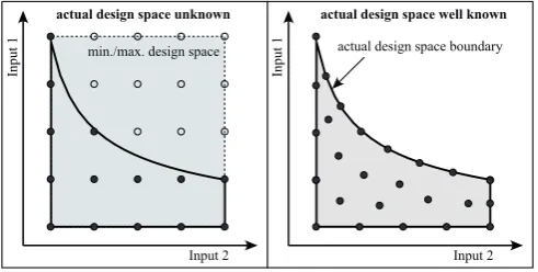
For all DoE strategies, especially the ones based on active learning, it is important to know the design space. Only if the design space is known the measurement points can be placed inside it in an optimal way. Moreover, the design space boundary itself is of particular importance. Since often optima will be found exactly on this boundary it is necessary to place measurements there. This is illustrated for a somewhat exaggerated example in Fig. 1. In the left diagram the design space is unknown, only the allowed minimum and maximum values of the individual inputs (e.g. actuating variables) are defined. With this information only a rectangular design space can be assumed and 25 mea-surement points are distributed equally inside the rectangular boundary. Not until the measurements are actually performed it turns out that 11 of the measurements are not feasible (circles) and only 14 measurements remain (dots) that can actually be used for modeling. Moreover, only 3 points lie close to the upper nonlinear boundary. If the design space was known (right diagram), all 25 points could be placed inside it and also exactly on the upper nonlinear boundary.
One common method to describe the design space bound-ary is placing a convex hull of hyperplanes around it [7]. This usually leads to a quite rough description of the design
min./max. design space actual design space boundary
In
put
1
Input 2 Input 2
In
put
1
actual design space unknown actual design space well known
[image:1.595.304.550.623.747.2]space and can become numerically demanding for high input dimensions. The alternative proposed in this paper is the use of support vector machines (SVM), which can robustly clas-sify even very complex sets of data. SVMs can produce very flexible boundaries and can handle large input dimensions well. Therefore a design space exploration algorithm based on an SVM is presented in this paper. Here the SVM not only describes the boundary, but is also iteratively used to find new measurement points and therefore constitutes an DoE algorithm for the determination of the design space.
C. Structure of the Paper
The following Sec. II introduces the topic of design space exploration. Sec. III presents the basics of using SVMs for linear and nonlinear classification problems. Sec. IV proposes a new method for iterative determination of the design space based on SVMs. Sec. V concludes the paper with a summary and an outlook on future work.
II. DESIGNSPACEEXPLORATION
The task of design space exploration is the determination of the design space by systematically changing the inputs of the system while detecting all possible constraint violations. Applied to the field of combustion engines this means that the actuating variables have to be changed carefully to avoid damage to the engine, but also quickly to reduce valuable measurement time. A basic method suitable for design space exploration is shown in Fig. 2.
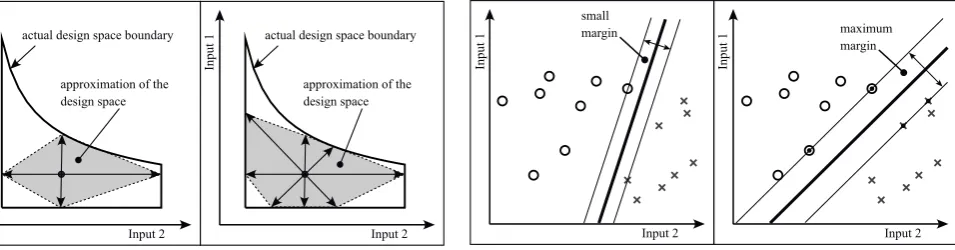
Starting from a safe point one input is changed at a time, in every direction, until a constraint is slightly violated. As the left diagram shows, the found points on the boundary are then connected by a polygonal line, or (hyper-)planes in higher input dimensions, constituting a convex hull. Since this is only a rough approximation the procedure is repeated, but by changing more than one input at once. As an ex-ample the right diagram in Fig. 2 shows an improvement of the approximation by using search directions rotated by 45◦. Using additional directions and different starting points further improvement can be achieved, but clearly the number off possible search directions explodes for higher input dimensions and the determination of the hull becomes computationally demanding.
A method that is based on the previously described idea, but is more sophisticated, is actually used for automotive applications (Rapid Hull Determination Algorithm [8]). In
approximation of the design space actual design space boundary
approximation of the design space actual design space boundary
In
put
1
Input 2 Input 2
In
put
[image:2.595.69.547.632.757.2]1
Fig. 2. Approximation of the design space through polygonal line (convex boundary). Left: Axis parallel search. Right: Additional 45◦directions.
Sec. IV an alternative method for design space exploration will be presented that avoids some of the previously men-tioned disadvantages. Since the method is based on SVMs an introduction on this topic is given in the following section.
III. SUPPORTVECTORMACHINES
For linear problems factor analysis or principal component analysis (PCA) are well established methods for handling high dimensional data and performing dimensionality reduc-tion, e.g. as preprocessing tools for solving classification problems. For nonlinear problems support vector machines, first conceived by [9], are a popular and powerful tool for classification. Detailed information can e.g. be found in [10]. While the use of SVMs has also been extended to regression problems, here only the classification abilities will be discussed further. The idea behind using SVMs for classification is to find a very robust classifier. This feature can be explained best using a linear SVM to separate linear separable classes of data.
A. Linear Classification Problem
The functional principle and the robustness aspect behind SVMs can be understood from the example in Fig. 3. Both diagrams show two classes of data points (marked by circles or crosses), which can clearly be separated by a line. However, the position and slope of the line can be varied in a wide range and still separate the classes.
The left diagram shows the choice of a line with a rather large slope. While separating the classes, the margin around the line, which is free of data points, is rather small. Therefore new data is likely to be misclassified, the classification is not very robust. The right diagram shows a line choice with a larger margin, calculated using a SVM. In fact, this is the line with the maximum margin possible, based on the given data. The robustness against misclassification is therefore maximized.
A closer inspection of the right diagram reveals that 2 circles and 2 crosses lie exactly on the margin (marked by a small dot). These points are calledsupport vectors, because only these points are needed to calculate the classification function, which is defined as a (hyper-) plane. The separating line is defined as the zero-crossing of this plane:
wT ·x+b= 0 (1)
where x = [x1, x2. . . xq]T are the coordinates of the data points (with q inputs) and the parameters wT =
In
put
1
Input 2 Input 2
In
put
1
small
margin maximum
margin
[image:2.595.48.303.633.755.2][w1, w2. . . wq]as well asbhave to be determined as follows. If training pointsxi (i= 1. . . N) are labeled eitheryi= +1 or yi=−1 depending on their class membership,w andb have to be selected in a way that following equation holds:
wT·xi+b≥+1 if yi= +1
wT·xi+b≤ −1 if yi=−1
⇒yi(wT·xi+b)−1≥0 ∀i
(2)
which means that the classification function is either +1or
−1 for points lying exactly on the margin borders (support vectors) for the respective classes. For points outside the margin the function has to be larger than+1or smaller than
−1 depending on the class.
For the case that the equality holds, meaning that only the support vectors are considered, it can be shown that the margin width is equal to ||w||−1. Therefore, to obtain the maximum margin ||w|| has to be minimized under the constraint yi(wT ·xi+b) ≥ 0. A quadratic optimization problem is obtained by solving min12||w||2 instead.
To solve the constrained problem Lagrange multipliersα
(withαi≥0) have to be introduced:
LP =
1 2||w||
2−α[y
i(xi·w+b)−1]
=1 2||w||
2− N
X
i=1
αiyi(xi·w+b) + N
X
i=1
αi (3)
Calculating ∂LP
∂w = 0 and
∂LP
∂b = 0 leads to the optimal values for the parametersw andb:
w=
N
X
i=1
αiyixi, N
X
i=1
αiyi= 0 (4) It is easier to solve the so calleddual formof this optimiza-tion problem, which depends on the Lagrange parameters
α and has therefore to be maximized instead of minimized. This form is gained by substituting (4) into (3):
LD= N
X
i=1
αi−
1 2
X
i,j
αiαjyiyjxTixj
s.t. αi ≥0, N
X
i=1
αiyi= 0
(5)
With Hij = yiyjxTi xj the dual form of the optimization problem can be finally written as:
max
α
"N
X
i=1
αi−
1 2α
THα
#
, αi>0, N
X
i=1
αiyi= 0 (6) Since this is a convex quadratic optimization problem (with linear constraints) it can be efficiently solved usingQuadratic Programming(QP). Whilew can be directly determined by using the optimal α and (4), the parameter b has to be calculated from the condition that for a support vector xs (pointxiwithαi>0), with corresponding classificationys, the classification function equals 1:
ys(wT·xs+b) = 1⇔b=
1
ys
−wT ·xs (7)
To gain a more robust value, usually b is calculated for all support vectors and the mean value is used.
[image:3.595.339.511.49.315.2] [image:3.595.51.291.323.459.2]Input 2
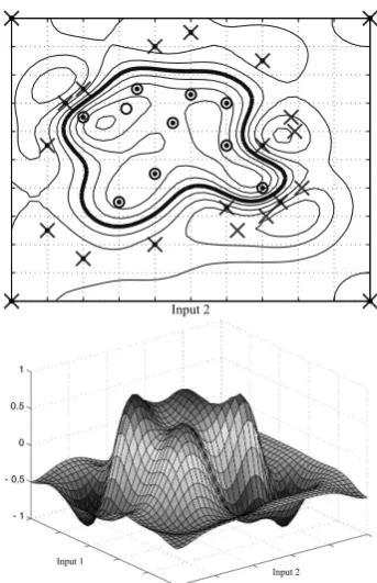
Fig. 4. Classification of a nonlinearly separable class usingRadial Basis Kernels. Top: Classification boundary (thick line, value of classification function equals zero) and contour lines of the classification function. Bottom: 3d plot of the classification function.
The optimization problem is not solvable if the data points are not linearly separable. In this case it is possible to calcu-late an approximate solution, which allows misclassification, using slack variables in the optimization problem. Also the SVM method can be extended to classification problems with more than two classes and can even be used for regression. These aspects are discussed e.g. in [11].
B. Nonlinear Classification Problem
Fig. 4 shows an example where the data points cannot be linearly separated, but a classification is still possible by using a suitable transformation x → ϕ(x). The resulting classification function for the example is shown in the lower diagram. Again the line separating the classes is defined by the zero-crossing of the classification function.
Both solving the optimization problem (eq. 5) and cal-culating the classification function (inserting w from eq. 4 in eq. 1) demands only for the dot product of the input vectorsxTixj→ϕ(xi)·ϕ(xj)to be known, notϕ(x)itself. The dot product is now replaced by a scalar kernel function
k(xi,xj) =ϕ(xi)·ϕ(xj). This procedure, often called the Kernel Trick, re-maps the data into a (potentially infinite dimensional) feature space where the separation is possible. Several kernel functions are suitable for this task. One of the most commonly used, besides the previously discussed Linear KernelxT
i xj, is the Radial Basis Kernel:
k(xi,xj) =e−
(x
i−xj)T(xi−xj)
2σ2
(8)
Input 2
safe point current point allowed point forbidden point new proposed point
design space boundary
In
put
1
Input 2
In
put
1
local search only
no success:
restart from safe point candidate points
currently estimated design space boundary
local search only
Input 2
1)
2)
3)
[image:4.595.51.550.51.386.2]4)
5)
6)
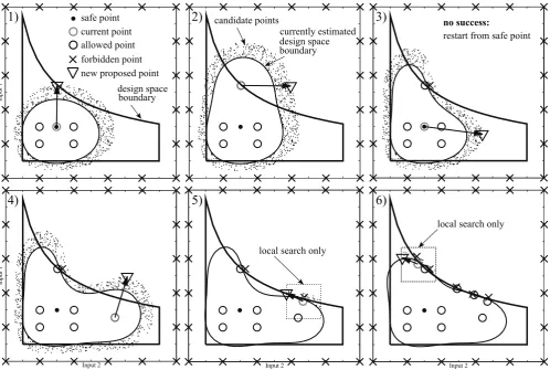
Fig. 5. Example for design space exploration. 1): Step 1 (successful). 2): Step 2 (unsuccessful, no allowed point found, return to safe point). 3): Step 3 from safe point (successful). 4): Step 4 (unsucessful, last allowed point will be used). 5): Step 5 (local search activated). 6): Step 9 (local search activated).
Since every point of the classification problem constitutes a constraint in the quadratic optimization problem (6) the calculation of the solution can be tedious when the number of points is very large. In this situation it is expedient to calcu-late only an approximate solution usingleast squares support vector machines (LS-SVM). In this case, only a system of linear equations has to be solved. WithΩij=yiyjk(xi,xj), y = [y1, y2, . . . , yN]T and1= [1,1, . . . ,1]T (N elements) it follows:
0 yT
y Ω+γI
b
α
=
0
1
(9)
where I is the unity matrix (dimension N ×N) and γ a ridge regression parameter, which balances the amount of misclassification against the condition of the matrix and has to be chosen suitably. For more details see [12], [13].
Finally, the advantages of using SVMs for classification can finally be summarized as follows:
1) Generation of almost arbitrary, non-convex boundaries. 2) The optimization problem is independent on number
of input dimensions (dot product).
3) Computational effort increases moderately with num-ber of points (measurements).
4) An approximate solution through a linear problem (LS-SVM) e.g. for time-critical applications is possible.
These advantages are the motivation to use SVMs for de-sign space exploration using the algorithm described in the following section.
IV. ALGORITHMBASED ONSVM
A. Functional Principle
To use SVMs for design space exploration some already classified points are needed right from the start. These points have not necessarily to be measured, it only has to be certain that their classification as either inside (allowed) or outside (forbidden) the design space is known. An example of the start configuration is shown in diagram 1 of Fig. 5. Forbidden points are placed here on a box around the actual design space. If the investigated system is e.g. a combustion engine, this box constitutes the individual (mechanical) limits of the actuating variables of the engine, which can’t be exceeded (e.g. throttle 0-100%). Also some allowed points have to be defined. In the case of a combustion engine, safe points for the actuating variables are known for every operating point. The allowed points could be placed close to such a safe point. With these points a classification boundary can be cal-culated as a first approximation of the design space. As diagram 1 in Fig. 5 shows this approximation covers only a small portion of the actual design space and therefore has to be improved by adapting iteratively to new measurements. The overall procedure, illustrated in Fig. 5, is as follows:
1) Begin in (or return to) safe starting point. 2) Calculate boundary from available measurements. 3) Calculate next measurement point.
6) If allowed point existed, proceed from this point with step 2), otherwise return to step 1).
The important question is how the new measurement point is selected. To gain a fast expansion of the approximated design space a large number of candidate points (marked by small dots in Fig. 5) are randomly placed inside a band around the currently approximated boundary, from which the new point will be selected. The speed of the expansion can be influenced by defining how far the band reaches outside the current boundary. Extending the band also to the inside of the boundary generates a more uniform and dense distribution of measurement points if needed. This effect is illustrated by an example in section IV-B.
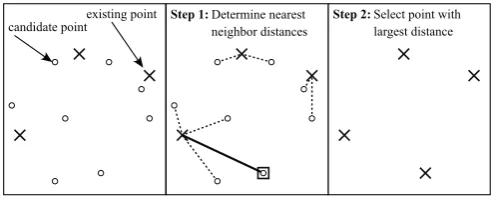
To spread the new points in few iterations throughout the design space the new measurement point is always selected from the candidate points as the point with the largest nearest neighbor distance. Fig. 6 shows that for all candidate points the closest already existing measurement point is determined (middle diagram, dashed lines). The candidate point with the largest distance to its closest neighbor is selected as new measurements point.
Another important issue is how the new point is ap-proached. To avoid engine damage the engine’s actuating variables are changed slowly and usually in small discrete steps. After each step the procedure is halted for a certain time to reach a steady state. This is especially important if the design space is restricted by temperature limits. If the new point is reached without violating any constraints, the procedure is repeated with the new point as starting point (Fig. 5, diagrams 2, 4). If during the approach a constraint is violated the last point which caused no violation and the point causing a violation are classified accordingly and stored. The procedure is then repeated from the not violating point (Fig. 5, diagram 5).
If the starting point for the next approach is already close to the actual design space border (Fig. 5, diagram 2) it is possible that no allowed measurement can be found at the next discrete step of the actuating variables. In this situation the algorithm returns to the defined safe point and starts from there again (Fig. 5, diagram 3).
The exact procedure of how the new measurement points should be approached depends strongly on the dynamic behavior of the examined system and has to be developed individually for this system. Usually two conflicting issues have to be balanced in this situation. On the one hand the new measurement points should be approached slowly to make sure that the measurement is not heavily influenced by dynamic effects and is at least close to the actual steady state. This is not only necessary to gain correctly classified data, but also to reduce the danger of large unnoticed constraint violations and therefore possible damage to the system. On the other hand, measurement time on a test bench is usually expensive and therefore should be minimized.
Another aspect that has to be addressed is that the pre-sented algorithm can freely chose a new measurement point from the candidate points independently from the last mea-surement, causing the algorithm to jump over large distances across the input space. This is not necessarily desirable during actual experiments, because such behavior leads to large changes in the state of the system. As a consequence it can take a long time until the steady state is reached again,
existing point candidate point
Step 1: Determine nearest Step 2:
neighbor distances
[image:5.595.303.551.52.151.2]Select point with largest distance
Fig. 6. Determination of new measurement point: Point with largest nearest neighbor distance.
which slows down the measurement process. Therefore a mechanism is included that prefers a more local search in certain situations by considering only candidate points in the vicinity of the current position. This is illustrated by the dashed box in diagrams 5 and 6 in Fig. 5.
B. Assessment of the Algorithm and Possible Improvements
In the left diagram of Fig. 7 the result of the design space exploration after about 40 measurements is depicted. The approximated design space is a good representation of the actual one. It can be seen that the algorithm places the points closely around the design space border and only sparsely inside the design space, which constitutes an economical use of the available measurements. The reverse, and not desirable, behavior can be seen in the right diagram where a different candidate point placement strategy was used: the candidates were always placed at the inside of the current boundary. The center diagram shows the first step of this exploration run as an example.
It can also be seen in Fig. 7 that some points at the border very close to each other are not classified correctly. This is caused by the use of a LS-SVM, which is only an approximation of the classification problem. Furthermore, at some places, especially the corners of the actual design space, the measurements are placed very closely. This is not desired and an improvement of the algorithm to avoid this behavior should be found.
It has also to be considered that some inputs may be changed faster and over a larger interval than others, since their influence on the process is smaller or less critical for constraint violations. This means that it would be advan-tageous to include a preference for certain input directions in the algorithm. This could e.g. be done by weighting the directions when calculating the nearest neighbor distances as depicted in Fig. 6.
So far the algorithm stops after a given number of measurements. This is a straightforward approach since the overall measurement time and therefore the budgeted costs for a test bench trial are usually known in advance. Hence the maximum number of measurements can be calculated and the iterative algorithm, which improves the approximated boundary with every new measurement, delivers the best approximation for the given costs. It would be desirable though to find an exit condition depending on the current quality of the approximated design space to reduce the number of measurements as much as possible for a given quality.
Input 2 Input 2
In
put
1
Input 2
current design space filled
with candiate points
candiate points only at the
[image:6.595.51.549.52.221.2]current design space border
Fig. 7. Example for design space exploration (result after about 40 steps). Left: Candidate points placed always at current design space border (as shown in Fig. 5). Center and right: Candidate Points placed always inside the current design space
false classification
1) 2) 3) 4)
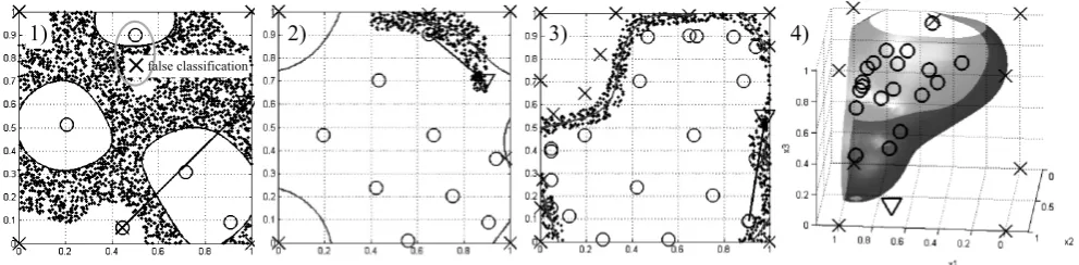
Fig. 8. Examples from test bed experiments: 1) Problems with too small standard deviation for the SVM kernels and false classification, because of too fast measurements. A good example of the procedure can be seen in 2) (beginning) and 3) (close to the end). 4) illustrates an example with 3 inputs.
Diagram 1) illustrates the problems that can occur. The standard deviation of the kernel functions was chosen to small. Also the waiting period between measurements was not long enough for the (dynamic) process to settle, causing misclassifications. Both factors caused (unrealistic) discon-tiguous areas. The diagrams 2) and 3) show a good working procedure near the start and end respectively. Diagram 4) is an example for a design space exploration with 3 inputs.
V. CONCLUSIONS ANDFUTUREWORKS
This paper presents an algorithm for design space explo-ration using support vector machines. The algorithm can ap-proximate not only convex, but also non-convex boundaries of the design space. The algorithm is numerically sound and independent on the number of input dimensions. The numerical effort increases moderately with the number of measurements. The results so far are very promising. The method was not only tested in simulations, but first tests were performed using an actual combustion engine.
The engine tests so far were focused on feasibility, but future work will of course comprise comparisons with other methods to achieve a more quantitative assessment. Further important aspects are the avoidance of close point placement, development of a better exit condition and the possibility to influence the measurement placement depending on the properties of the inputs, e.g. allowing large changes only for uncritical inputs.
REFERENCES
[1] L. Kn¨odler, Methoden der restringierten Online-Optimierung zzur Basisapplikation moderner Verbrennungsmotoren. Berlin, Germany: Logos, 2004.
[2] R. Isermann (Hrsg.),Modellgest¨utzte Steuerung, Regelung und Diag-nose von Verbrennungsmotoren. Springer, 2003.
[3] K. R¨opke (Ed.),Design of Experiments (DoE) in Engine Development II. Expert-Verlag, 2005.
[4] D. C. Montgomery,Design and Analysis of Experiments. John Wiley & Sons, Inc., USA, 2005.
[5] G. Schohn and D. Cohn, “Less is more: Active learning with support vector machines,” in Proceedings of the Seventeenth International Conference on Machine Learning. Morgan Kaufmann, 2000, pp. 839–846.
[6] B. Hartmann, T. Ebert, and O. Nelles, “Model-based design of experiments based on local model networks for nonlinear processes with low noise levels,” inAmerican Control Conference (ACC), 2011, 29 2011-july 1 2011, pp. 5306 –5311.
[7] B. Bradford, D. David, and H. Hannu, “The quickhull algorithm for convex hulls,”ACM Transactions on Mathematical Software, vol. 22, pp. 469–483, 1996.
[8] P. Renniger and M. Aleksandrov, “Rapid hull determination: a new method to determine the design space for model based approaches,” inDesign of Experiments (DoE) in der Motorenentwicklung, Berlin, Germany, June 2005.
[9] C. Cortes and V. Vapnik, “Support vector networks,”Machine Learn-ing, vol. 20, no. 3, pp. 273–297, 1995.
[10] B. Sch¨olkopf and A. Smola,Learning with kernels: Support vector machines, regularization, optimization, and beyond. MIT Press, 2002. [11] C. Bishop,Pattern Recognition and Machine Learning. Springer,
2006.
[12] J. Suykens and J. Vandewalle, “Least squares support vector machine classifiers,”Neural processing letters, vol. 9, no. 3, pp. 293–300, 1999. [13] J. Suykens,Least squares support vector machines. World Scientific
[image:6.595.51.547.265.387.2]