Abstract—A novel family of explicit method is presented. Unlike conventional integration methods, the coefficients of the two difference equations are no longer constant but functions of the initial structural properties of the system analyzed and the size of integration time step. The most important properties of the proposed family method are the second-order accuracy, the possibility of unconditional stability and the explicitness of each time step. The possibility of unconditional stability in addition to the second-order accuracy will allow using a large time step for conducting the step-by-step integration; and the explicitness of each time step involves no iterative procedure. As a result, many computational efforts can be saved when compared to currently available integration methods.
Index Terms—accuracy, explicit method, nonlinear systems, stability, step-by-step integration, structural dynamics
I. INTRODUCTION
WO difference equations are needed in establishing an integration method. One is for displacement increment and the other is for velocity increment [1-6]. In general, the coefficients of the two difference equations are some specific constants. Since the numerical properties of an integration method are highly dependent upon the structural properties of the system analyzed, a brand new concept was proposed by using coefficient matrices, which are functions of initial structural properties and step size. Apparently, an integration method of this type is structure-dependent. As a result, two family methods were developed by Chang [7-8]. In general, they are conditionally stable, second-order accurate, explicit, one-step methods, and have favorable numerical dissipation which can be continuously controlled and it is possible to achieve zero damping. Since they can only have conditional stability, their applications are very limited. Consequently, some unconditionally stable, explicit methods [9-12] which are also structure-dependent were developed to overcome this difficulty. The integration of the unconditional stability and second-order accuracy will allow using a large time step; and the explicitness of each time step leads to no nonlinear iteration. Thus, many computational efforts are saved when compared to the currently available integration methods.
Only the difference equation for displacement increment is
Manuscript received December 18, 2011. This work was supported by the National Science Council, Taipei, Taiwan, ROC under Grant NSC-99-2221- E-027-029.
Shuenn-Yih Chang is with the Department of Civil Engineering, National Taipei University of Technology, Taipei, 10608, Taiwan, ROC. (e-mail: [email protected]).
Chiu-Li Huang is with Fu Jen Catholic University, New Taipei City 242, Taiwan, ROC. (e-mail: [email protected]).
structure-dependent while that for velocity increment still involves constant coefficients for the currently developed structure-dependent integration methods [9-12]. In this paper, a new family of explicit methods is proposed, whose two difference equations are both structure-dependent. This family method simplifies the equation for computing velocity after obtaining displacement and thus further computational efforts can be saved. Numerical properties of this family method will be analytically studied. Numerical examples will be used to examine analytical results and the computational efficiency of this proposed family method is also explored.
II. PROPOSED FAMILY METHOD
The equation of motion for a discretized, single degree of freedom system can be expressed as
f ku u c u
m (1)
where m, c, k and f representthemass, viscous damping coefficient, stiffness and external force, respectively; and u, u and u denote the displacement, velocity and acceleration, respectively. The initial-value problem is to solve (1) to meet the given initial conditions.
Although many integration methods can be employed to solve (1) a new family of explicit methods is proposed and it can be expressed as:
1 1 1 1 2 1
1
i i i i
i i i i
i i i
ma cv kd f
d d t v t a
v v t a
(2)
where
22
0 0 0 0
1
1 2
m
m t c t k
(3)
where 0 0
t and 0 k0/m is the natural frequencyof the system determined from the initial stiffness of k0;
0 2 0
c m, which is assumed that the viscous damping ratio is determined from the initial structural properties. Unlike a general integration method, it is interesting to find that the coefficient is no longer a given constant but depends on the initial structural properties and step size. Noticed that is proposed to be invariant in a whole step-by-step integration procedure. The parameters and generally control the numerical properties of the proposed family method.
Structure-Dependent Integration Algorithms for
Time History Analysis
Shuenn-Yih Chang and Chiu-Li Huang
III. NUMERICAL PROPERTIES
To assess the numerical properties of the proposed family method, its computing sequence within a single time step must be reflected in the analysis. The stiffness in the first line of (2) may vary not only from step to step but also within a time step for nonlinear systems. Hence, this characteristic must be considered in the basic analysis. For this purpose, the symbol ri is introduced to represent the restoring force at the end of the (i)th time step and is expressed as rikidi, where ki is the stiffness at the end of the (i)th time step.
The actual computing sequence of the (i)th time step for the proposed family method can be written in a recursive matrix form as:
1 1 1
1
i i i i
i A X L f
X (4)
where
T 1 21 1
1 , ,
i i i i d tv t a
X ; and Ai1 and Li1 are the
amplification matrix and the load vector for the (i1)th time step, respectively. The computing sequences of di1, vi1
and ai1 for the (i1)th time step can be explicitly obtained.
As a result, the explicit expression of the amplification matrix is found to be:
2 0 0 1 2 0 0 22 2 0 1
1 0 1 2
0 0 1 1 1 1 2 1 0 1 1 2 2 2 1 2 i i i i
A (5)
The characteristic equation of this matrix can be computed by using Ai1I 0. As a result, it is found to be
0
2 2 1
3
A A (6)
where
2 2
0 0 1
1 2 0 0 2 0 0 2 2 0 0
2 2 1 2 2
1 2
1 2 1
1 2 i A A (7)
where 2
0 1 2
1
i i since i1ki1/k0 and i1i1(t) , in
which i1 ki1/m is defined. It is implied by i11 that
the instantaneous stiffness at the end of the (i1)th time step is equal to the initial stiffness. Whereas, i11 is used to
denote a case of instantaneous stiffness hardening at the end of the (i1)th time step, where the instantaneous stiffness
1
i
k is larger than the initial stiffness k0, and a case of
instantaneous stiffness softening can be denoted by i11,
where the instantaneous stiffness ki1 is less than the initial
stiffness k0 .
A. Stability
In the following stability analysis, a zero viscous damping ratio is assumed since it is complicated to obtain an analytical expression of the stability limit for nonzero viscous damping. It is advisable to satisfy the stability conditions by restricting the two eigenvalues of Ai1 to be complex conjugate in
addition to (Ai1)1, where (Ai1) is the spectral radius of 1
i
A at the end of the (i1)th time step.
As a result, the stability conditions for the proposed family method are found to be:
1 4 0 1 1 4
0 0 1
1 4 1
0 if
1
0 if
i u i i (4)
where 0
u
is referred to be the upper stability limit. It is clear that the proposed family method is unconditionally stable as
1
4 i1
while it becomes conditionally stable as
1
4 i1
.
Some members of this family method are of great interest and will be studied next. The symbols of PFM1, PFM2 and PFM3 are used to represent the members of the proposed family method with 0, 1/4 and 1/2, respectively, in addition to
1 / 2
[image:2.595.49.292.360.452.2] .
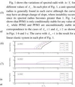
Fig. 1 shows the variations of spectral radii with t T/ 0 for
different values of i1. In each plot of Fig. 1, a unit spectral
radius is generally found in each curve although the curve may have an abrupt change of slope, where instability occurs since its spectral radius becomes greater than 1. Fig. 1-a shows that PFM1 is only conditionally stable for any value of
1
i
while PFM2 and PFM3 are unconditionally stable in correspondence to the cases of i11 and i12 as shown
in Figs. 1-b and 1-c. The curve with i11 is the result for a
linear elastic system in each plot of Fig. 1.
Fig. 1. Variations of spectral radius with t T/ 0 for different members of the
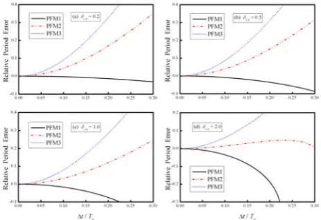
proposed family method B. Accuracy
Variations of relative period errors with t T/ 0 are shown
in Fig. 2. It is found that the absolute relative period error, in general, increases with the increase of t T/ 0 as i1 and
[image:2.595.282.548.361.669.2]insignificant difference as t T/ 00.05. This implies that
each integration method can provide a reliable solution with comparable accuracy, if t T/ 00.05 is met for the modes of
interest. The results for a linear elastic system are shown in Fig. 2-c since the case of i11 is considered in this plot. In
[image:3.595.53.285.177.336.2]general, PFM1 will lead to period shrinkage while period elongation is found for PFM2 and PFM3. It is also found that period distortion increases with the increase of for a given value of t T/ 0.
Fig. 2. Variations of relative period errors with t T/ 0 for different i1,
where T0 is the natural period determined from initial structural properties.
It is found that there is no numerical dissipation [11-12, 17-18] for the proposed family method for a zero viscous damping ratio since A21 which is manifested from the second line of (7).
IV. IMPLEMENTATION FOR MULTIPLE DEGREE OF FREEDOM SYSTEM
After obtaining the numerical properties of the proposed family method, it is of great interest to confirm the analytical results and study computational efficiency. For this purpose, an implementation of the proposed family method is sketched, and it can be written as:
1 1 1 1 2 1
1
i i i i
i i i i
i i i
t t
t
Ma Cv Kd f
d d v Ψ a
v v Ψ a
(8)
where Ψ is a coefficient matrix for a multiple degree of freedom system in correspondence to for a single degree of freedom system and is:
2 11 1
0 0
t t
Ψ I M C M K (9)
where C0 is the damping matrix, determined from the initial
structural properties, and K0 is the initial stiffness matrix. 0
C and K0 will remain invariant for a complete integration
procedure. A constant damping matrix is often assumed, i.e.,
0
C C , while the stiffness matrix K is, in general, different from the initial stiffness K0 for a nonlinear system.
The displacement vector is computed by using the second line of (8) and then the restoring force vector corresponding to this displacement vector is determined from an assumed force-displacement model. Thus, ri1 is used to replace Kdi1
to reflect the force-displacement relationship for a nonlinear system. The use of the second line of (8) to determine di1
can be alternatively written and it is numerically equivalent to solve the equation of:
2 2
0 0 i1 i i i
t t t t
M C K d d v M a (10)
Although the proposed family method can have an explicit implementation it requires solving this equation to yield the next step displacement vector for each time step. At first glance, it seems to consume more computational efforts when compared to a general explicit method since a triangulation and a substitution are needed if a direct elimination method is used. However, the triangulation of 2
0 0
t t
M C K is
needed to be conducted only once since it remains unchanged for a complete integration procedure if t is a constant in addition to the invariant of C0 and K0.
It is computationally efficient if vi1 does not obtain from
the third line of (8) since it involves a substitution for each time step. Alternatively, the vi1 can be determined by using
the following equation:
1 1
i i i
t
d d
v (11)
This relationship is simply derived from the second and third lines of (8) and it involves no substitution for each time step. Finally, the first line of (8) can be used to compute ai1 after
determining di1 and vi1.
V. NUMERICAL ILLUSTRATIONS
To verify the numerical properties of the proposed family method, some numerical examples are examined. On the other hand, in order to emphasize the advantages of involving no nonlinear iterations and the possibility of unconditional stability, the computational efficiency of the proposed family method is also studied through recorded CPU time in contrast to NEM and the well-known constant average acceleration method (AAM).
A. Example 1
A two-story shear building is considered. The floor beams and slabs of the structure are assumed to be flexurally rigid. The lumped masses are taken as 4
1 10
m kg and 5
2 10
m kg
for the bottom and top floors, respectively. To simulate different stiffness properties, the stiffness of each story is taken to be in the following form:
0 1
kk u (12)
where k0 is the initial stiffness and u is a story drift. The
general, the initial stiffness is taken as 8
0 10
k N/m for the bottom story while for the top story it is taken as 6
0 10
k
N/m. The natural frequencies of the structure are 3.15 and 100.50rad/sec based on the initial stiffness matrix. Notice that the system is intended to have a relatively high second mode so that the unconditional stability can be illustrated. To simulate a linear elastic system, an instantaneous stiffness softening system and an instantaneous stiffness hardening system, three different values of 1 and 2 are taken for the
nonlinear terms for the bottom and top stories. S1 12 0 linear elastic
S2 12 0.5 instantaneous stiffness softening
S3 12 0.5 instantaneous stiffness hardening
The three systems are excited by an acceleration of 10sin(5 )t at the base. The results obtained from NEM with t 0.001
sec are considered as reference solutions for comparison. Meanwhile, numerical results are also obtained from NEM with t 0.03sec , and PFM3 with t 0.06 sec .
Fig.3. Displacement response to base acceleration of 10 sin(5 )t for S1
Numerical results for S1 are shown in Fig. 3. The solutions obtained from NEM with t 0.03 sec become unstable in the very early response while those obtained from PFM3 with
0.06 t
sec are reliable. It is clear that instability is due to the violation of upper stability limit 2 if using NEM while unconditional stability is indicated by the solutions obtained from PFM3 since it remains stable for the value of 2
0
as large as 6.03 for the second mode. The response contribution from the second mode to the total response is insignificant since reliable solutions can be achieved for PFM3, where the first mode is accurately integrated while a significant period distortion is found in the second mode.
The displacement responses for S2 are shown in Fig. 4. In addition, the response time histories of relative period error, instantaneous degree of nonlinearity and upper stability limit are plotted in Fig. 5. Reliable solutions are obtained from PFM3 with t 0.06sec since the relative period error is small for the first mode, as shown in Fig. 5-a although the second mode shows significant period distortion as indicated in Fig. 5-b. Figs. 5-c and 5-d reveal that the instantaneous degree of nonlinearity of both modes are always less than or
equal to 1. Therefore, a stable computation can be achieved for PFM3 since they can have unconditional stability for an instantaneous stiffness softening system. Fig. 5-f reveals that the upper stability limit of the second mode is violated, where
2 2~
0 3.02 0
u
is found if using NEM with the time step of 0.03
t
sec . Hence, instability occurs. It is worth noting that no curves for PFM3 in Figs. 5-e and 5-f are because that the upper stability limit is infinite for an instantaneous stiffness softening system if using PFM3.
Fig.4. Displacement response to base acceleration of 10 sin(5 )t for S2
Fig.5. Response time histories to base acceleration of 10 sin(5 )t for S2
Fig. 6 shows the displacement responses for S3 and the corresponding response time histories of relative period error, instantaneous degree of nonlinearity and upper stability limit are plotted in Fig. 7. It seems that PFM3 with
0.06 t
sec gives acceptable solutions. This is because that the relative period error is small for the dominant first mode, as shown in Fig. 7-a, although a very large relative period error is found in the second mode, as shown in Fig. 7-b. However, the most important aspects are that PFM3 is unconditionally stable as i12 and both Figs. 7-c and 7-d
show that 1
i
and 2
i
are less than about 1.8. Since 1
i
and 2
i
are less than 2 there is no upper stability limit for PFM3 as shown in Figs. 7-e and 7-f. Since Figs. 7-c and 7-d show that 1
1 i
and 2
1 i
for the two modes, the upper stability limit for each mode for NEM is shrunk. As a result, the use of
0.03 t
sec leads to instability in the early response because 2 2~
0 3.02 0
u
illustrates the superiority of PFM3 in the step-by-step solution of a nonlinear system since it can have unconditional stability for a certain instantaneous stiffness hardening systems in addition to a linear elastic system and an instantaneous stiffness softening system.
[image:5.595.50.283.309.468.2]Fig.6. Displacement response to base acceleration of 10 sin(5 )t for S3
[image:5.595.311.544.351.405.2]Fig.7. Response time histories to base acceleration of 10 sin(5 )t for S3
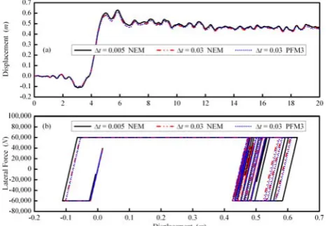
Fig. 8. Displacement responses to TCU075 and corresponding hysteretic loops for PFM3
B. Example 2
A single degree of freedom system with an elastoplastic behavior is considered in this example. The lumped mass and the stiffness for the system are taken to be 4
4 10 kg and
6
2.56 10 N/m , respectively. The initial natural frequency is found to be 8 rad/sec . The yielding strength is assumed to be
4
6 10 N for both tension and compression. The system is subjected to the ground acceleration record of TCU075 with a peak ground acceleration of 0.5g. TCU075 is a near-fault ground motion record and was collected by the Central Weather Bureau during the Chi-Chi earthquake.
Numerical results are shown in Fig. 8. Numerical solutions obtained from NEM with a time step of t 0.005sec are considered as reference solutions for comparisons. Both NEM and PFM3 with the time step of t 0.03sec , which corresponds to t T/ 00.04 , are used. In Fig. 8-a, the
displacement responses obtained from NEM and PFM3 are very close to the reference solutions. A slight difference between the results obtained from NEM and PFM3 and the reference solutions might be due to the fact that the yielding point is not exactly captured. It is apparent that the pulse-like wave has significant influence on the seismic response of the structure, because it imposes high seismic energy on the structure.
C. Example 3
To study the computational efficiency of the proposed family method, a n-degree-of-freedom spring-mass system as shown in Fig. 9 is considered.
Fig. 9. A n-degree of freedom spring-mass system
The structural properties of the system are selected to be
2
10 kg i
m and 7
21
10 1 N/m
i i i
k u u for i1,,n. Although a zero damping ratio is assumed in this example a viscous damping matrix is included in the equations of motion for completeness. The system is excited by harmonic load of sin(t) at the free end. The n values of 500, 1000 and 2000 are chosen so that the systems with 500-DOF, 1000-DOF and 2000-DOF are simulated. The lowest natural frequency is 3.14 rad/sec for the 500-DOF system before the system deforms. Similarly, it is found to be 1.57 and 0.785 rad/sec for the 1000-DOF and 2000-DOF systems. The highest natural frequency is found to be 2000.00 rad/sec for all the three systems. NEM, AAM and PFM3 are applied to compute the displacement responses. Since the highest natural frequency is as large as 2000.00 rad/sec the time step of t 0.001sec is chosen to be used by NEM so that the stability condition can be satisfied. The numerical solution obtained from this time step can be considered as a reference solution since the time step is much smaller than that required by accuracy consideration.
The displacements of the largest degree of freedom for the 500-DOF, 1000-DOF and 2000- DOF systems are shown in Fig. 10. AAM and PFM3 give accurate solutions for the 500-DOF system if t 0.05 sec is used. Meanwhile, they also lead to reliable results for the 1000-DOF system if using
0.10 t
[image:5.595.52.286.500.661.2]stability for instantaneous stiffness softening systems since the product of the time step and the highest natural frequency is as large as 100 for the 500-DOF system, 200 for the 1000-DOF system and 300 for the 2000-DOF system.
Fig. 10. Displacement responses for 500-DOF, 1000-DOF and 2000-DOF spring-mass systems
The CPU time consumed in each dynamic analysis for using NEM, AAM and PFM3 is recorded. As a result, Table I summarizes the recorded CPU time for all the analyses. For brevity, the CPU time consumed by NEM with t 0.001
sec is denoted by (NEM)
CPU . On the other hand, the symbols
of (AAM)
CPU and (PFM3)
CPU are introduced to denote the CPU time consumed for using AAM and PFM3, respectively. It seems that the time step of 0.05 sec is the largest allowable time step to yield reliable solutions for the 500-DOF system while those of 0.10 sec and 0.15 sec are for the 1000-DOf system and 2000-DOF system, respectively.
TABLEI.COMPARISON OF CPUTIME
The 4th column of Table I reveals that the CPU time consumed by PFM3 for each system is much smaller than that for NEM or AAM, which is shown in the 2nd and 3rd columns. NEM is computationally inefficient to solve this type of problems since it can only have conditional stability and thus the upper stability limit is a very stringent limitation in selecting an appropriate time step for the high frequency of 2000 rad/sec . In fact, a time step of t 0.001sec is needed to meet the upper stability limit for the three different systems if using NEM. Although AAM has unconditional stability and a large time step can be selected based on accuracy consideration it still consumes many computational efforts. This is because an iteration procedure is generally needed in each time step for an implicit method and it is very time consuming for a matrix of large order.
The explicitness of each time step and the unconditional stability explain why PFM3 can save many computational efforts. The explicitness of each time step allows PFM3 involve no nonlinear iterations and the unconditional stability allow it select an appropriate time step without considering the upper stability limit.
Columns 5 and 6 reveal that the ratio of the CPU time consumed by PFM3 over that consumed by NEM or AAM decreases with the increase of the total number of the degree of freedom. This implies that the computational efficiency of PFM3 becomes more significant for a system with a large number of the degree of freedom when compared to NEM and AAM. Both the 5th and 6th columns show that the ratio of the CPU time is smaller than 1% and consequently the saving of computational efforts is very significant for PFM3.
VI. CONCLUSIONS
A novel family of structure-dependent explicit methods is presented. It can have unconditional stability if 1
4 i1
is
chosen. Whereas, it becomes conditional stable as 1
4 i1
is
used. In general, the proposed family method is second-order accurate and has no numerical dissipation for 1 / 2. For the proposed family method, it is very promising to choose PFM3 for practical applications since it has second-order accuracy and the possibility of unconditional stability for nonlinear systems. PFM3 seems very competitive with other integration methods for solving a general structural dynamic problem, whose responses are dominated by low frequency modes. This is because it can integrate the unconditional stability and the explicitness of each time step. Hence, it can save many computational efforts when compared to a conditionally stable explicit method, where the step size is limited, and an implicit method, where an iterative procedure is often needed.
REFERENCES
[1] K. J. Bathe, “Conserving energy and momentum in nonlinear dynamics: A simple implicit time integration schemes,” Computers & Structures, vol. 85, pp.437-445, 2007.
[2] S.Y. Chang, “A series of energy conserving algorithms for structural dynamics,” Journal of the Chinese Institute of Engineers, vol. 19, no. 2, pp. 219-230, 1996.
[3] J. Chung and G. M. Hulbert, “A time integration algorithm for structural dynamics with improved numerical dissipation: the generalized-method,” Journal of Applied Mechanics, vol. 60, no. 6, pp. 371-375, 1993.
[4] H. M. Hilber, T. J. R. Hughes and R. L. Taylor, “Improved numerical dissipation for time integration algorithms in structural dynamics,”
Earthquake Engineering and Structural Dynamics, vol. 5, pp. 283- 292, 1977.
[5] J. C. Houbolt, “A recurrence matrix solution for the dynamic response of elastic aircraft,” Journal of the Aeronautical Sciences vol. 17: pp. 540-550, 1950.
[6] N. M. Newmark, “A method of computation for structural dynamics,”
Journal of Engineering Mechanics Division ASCE, vol. 85, pp. 67-94, 1959.
[7] S. Y. Chang, “Improved numerical dissipation for explicit methods in pseudodynamic tests,” Earthquake Engineering and Structural Dynamics, vol. 26, pp. 917-929, 1997.
[8] S. Y. Chang, “The function pseudodynamic algorithm,” Journal of Earthquake Engineering, vol. 4, no. 3, pp. 303-320, 2000. [9] S. Y. Chang, “Explicit pseudodynamic algorithm with unconditional
stability,” Journal of Engineering Mechanics ASCE, vol. 128, no. 9, pp. 935-947, 2002.
[10] S. Y. Chang, “An explicit method with improved stability property,”
International Journal for Numerical Method in Engineering, vol. 77, no. 8, pp. 1100-1120, 2009.
[11] S. Y. Chang, “Explicit pseudodynamic algorithm with improved stability properties,” Journal of Engineering Mechanics ASCE, vol. 136, no. 5, pp. 599-612, 2010.
[image:6.595.60.279.454.517.2]