Distributed Control of Heating, Ventilation and Air
Conditioning Systems in Smart Buildings
Najmeh Forouzandehmehr
Electrical and Computer Engineering Department
University of Houston Houston, Texas, USA [email protected]
Samir M. Perlaza
Department of Electrical Engineering
Priceton University Princeton, NJ, USA [email protected]
Zhu Han
Electrical and Computer Engineering Department University of Houston Houston, Texas, USA
H. Vincent Poor
Department of Electrical Engineering
Priceton University Princeton, NJ, USA [email protected]
Abstract—In this paper, the problem of distributed control of the heating, ventilation and air conditioning (HVAC) system in an energy-smart building is addressed. Using tools from game theory the interaction among several autonomous HVAC units is studied and simple learning dynamics based on trial-and-error learning are proposed to achieve equilibrium. In particular, it is shown that this algorithm reaches stochastically stable states that are equilibria and maximizers of the global welfare of the cor-responding game. Simulation results demonstrate that dynamic distributed control for the HVAC system can significantly increase the energy efficiency of smart buildings.
I. INTRODUCTION
Buildings consume almost 70% of the total electricity generated in the US [1]. One of the major energy-consuming systems of a building is the heating, ventilation and air con-ditioning (HVAC) system. More precisely, an HVAC system might exhaust more than 65% of the total electrical energy consumed by a building [2]. The high energy consumption of HVAC systems raises energy costs as well as environ-mental concerns. Therefore, a desirable capability of future “smart buildings” is energy reduction via fine-grained control of HVAC systems. For instance, an HVAC system can be conceived as an autonomous system that adjusts the indoor temperature of different locations in the building based on the occupancy [3].
A growing body of research suggests that efficient control of HVAC systems might significantly increase the energy efficiency of future smart-buildings. For instance, in [4], the authors explored the problem of computing optimal control strategies for time-scheduled operation taking into considera-tion building operaconsidera-tion schedules, e.g., night-setback, start-up and occupied modes, as well as a predicted weather profile. In [5], dynamic and real-time simulation models are developed to study the thermal, hydraulic, mechanical, environmental and energy performance of smart buildings. In [6], the authors presented a simulation tool, “QUICK Control”, to predict the This research was supported in part by the Army Research Office under MURI GrantW911N F-11-1-0036and the U.S. National Science Founda-tion GrantsCN S-1265268,CN S-1117560,ECCS-1028782andCN S
-0953377.
effect of changing control strategies on indoor comfort and energy consumption.
For occupancy-based control of HVAC systems, a funda-mental requirement is a sensor network to capture the occu-pancy changes in real time. In [7], the authors proposed several control strategies based on real time occupancy monitoring and occupancy predictions.
In this paper, tools from game theory and multi-agent learning are used to design a cost-efficient distributed control for HVAC systems. This work takes into consideration the electricity cost and predetermined ranges of desirable tempera-tures during certain periods for all locations in the building that are subject to temperature control. The main game-theoretic tool of this analysis is the notion of a satisfaction equilibrium (SE) [9]. Basically, an SE is an equilibrium concept in which players do not seek any benefit maximization but only the sat-isfaction of their own individual constraints. This equilibrium is thoroughly studied in the context of the distributed control of HVAC systems. More importantly, a simple algorithm based on the notion of trial-and-error learning [10] that is capable of achieving an SE is also presented.
The rest of this paper is organized as follows. Section II introduces the system model. Section III describes two games, one in the satisfaction form and another one in the normal form, to model the problem of distributed control of HVAC systems. Therein, a fully distributed learning algorithm is also provided to achieve the equilibria of the corresponding games. Section V presents some simulation results, and Section VI concludes this work.
II. SYSTEMMODEL
Consider a smart-building withnzones subject to tempera-ture control. Each zone is managed by an HVAC system that is fully independent of all the other HVAC units in the building. The goal is to reduce the electricity cost by dynamically adjusting the operation of the HVAC units such that two main constraints are satisfied:(i)The temperature of a given roomi, withi∈ {1, . . . , n}must be kept within a desirable range for certain predetermined periods; and(ii) The total power load dedicated for heating, ventilation and air conditioning must not exceed a predetermined threshold.
Consider that temperature is controlled with a granular-ity of 1 hour. At the beginning of the day, HVAC unit i chooses its own daily power consumption vector, denoted by, Li = (li(1), ..., li(t), ..., li(24)), where li(t) denotes the
power consumed by HVAC uniti at hourt. Each HVAC unit chooses its vector Li from a finite set of vectors denoted by
Li. The daily power consumption vector is selected in order
to minimize the daily electricity cost
Φ(L,P) = n
X
i=1 24
X
t=1
µi(li(t), p(t)), (1) where L = (L1, . . . ,Ln) ∈ L1 × . . . × Ln, P = (p(1), . . . , p(24)) ∈R24 , with p(t)the hourly market price
per energy unit. Note that the vectorPis assumed to be known by each HVAC unit at the beginning of the day. The function µi :Li×R→Rmodels the operation cost of HVACiwith
power load li(t)and pricepi(t). One example of the function µi is presented in [11]. Therein, the functionµi is defined as
follows:
µi(li(t), p(t)) =c1p(t)li(t)
2
+c2p(t)li(t) +c3, (2)
where c1, c2 and c3 are constant parameters that are
deter-mined based on experimental data. One of the advantages of a quadratic model for the operation cost of an HVAC unit is that it is more realistic and flexible than other models, e.g., the translog cost model [12].
The total power load allocated for the HVAC system satisfies the following constraint at each 1-hour periodt of the day:
∀t∈ {1, . . . ,24},
n
X
i=1
li(t)≤Lr, (3)
where the threshold valueLris imposed by the characteristics
of the power distribution feeder/bus of the building. This threshold is assumed to remain the same at each periodt.
The temperature Ti(t)of zone i during period t must fall within the interval[Tti,T¯t
i]. Note that this control is enforced
only during certain periods. Hence, the set Ii denotes the
periods over which this rule is enforced, i.e.,
∀t∈ Ii, Tti ≤Ti(t)≤T¯ t
i. (4)
For all the other periods t∈ {1, . . . ,24} \ Ii no temperature
control is performed. The indoor temperature is predicted up to
24 hours in advance using a simple exponential decay model proposed by [13]. That is,
Ti(t+ 1) =Ti(t) + (1−)(TOD(t)−γKli(t)), (5)
whereis the thermal time constant of the building;γis a fac-tor capturing the efficiency of the air conditioning unit to cool the air inside the building ; TOD is the outside temperature
which is predicted a day ahead; and K is a conversion factor that is proportional to the performance coefficient of the HVAC unit divided by the total thermal mass. The HVAC unit uses powerli(t)to control the temperature of zoneiduring period t. In this model, our focus is only on the cooling scenario. The results for a heating scenario can also be easily obtained
by changing the sign of−γKli(t). Equation (5) explains how the constraint (4) relates to the power consumed by the HVAC unit. The HVAC control units should select their consumption amounts in a way that the indoor temperature obtained from (5) falls within the comfort interval (4) and minimize the total cost in (1). That is, the vector L = (L1, . . . ,Ln) must be
chosen such that
min
L∈L1×...×Ln
n
X
i=1 24
X
t=1
µi(li(t), p(t)) (6)
s.t.
n
X
i=1
li(t)≤Lr, ∀t∈ {1, . . . ,24} and
Tit≤Ti(t)≤T¯it, ∀t∈ Ii.
The above problem can be solved at the beginning of the day such that the vectorLi= (li(1), ..., li(t), ..., li(24))is entirely
calculated by HVAC i only once per day; or at each period t, the HVAC determines its individual load li(t+ 1). Both
alternatives are studied in Section IV. III. GAMEFORMULATION
The distributed control problem of the HVAC system de-scribed above can be modeled via two games formulations: a game in normal form [14] and a game in satisfaction form [9].
A. Game in Normal Form
Consider the game in normal form
G= (N,L,{ξi}{i∈N }). (7) The set N = {1, . . . , n} represents set of players. HVAC i is represented by player i. The set of actions of player i is the set of daily power consumption vectorsLi. Hence, the set
of actions of the game isL=L1× L2×. . .Ln. The payoff
functionξi:L ×R24→Rof player iis defined by
ξi(L,P) = (8)
1
β+ 1 1−
P24
t=1µi(li(t), p(t)) 24µmax
+β1{Li∈fi(L−i)}
!
, whereβis a design parameter,µiis defined in (2) andµmaxis
the maximum cost userican experience. The correspondence fi :L1×. . .× Li−1× Li+1×. . .× Ln→2Li is defined as
follows:
fi(L−i) =
n
Li∈ Li:∀t∈ {1, ...,24} (9) n
X
i=1
li(t)≤Lr andTti ≤Ti(t)≤T¯ t i
o
. The payoff function in (8) captures the tradeoff between satisfying the individual constraints of playeriand minimizing the individual consumption cost. Note that increasing the value of β leads to the player focusing on in the satisfaction of its individual constraints. Alternatively, reducing the value of β leads the player to focus more on the reduction of the individual operating cost. This utility function was first proposed in [15] for the case of decentralized radio resource allocation in wireless networks.
An interesting outcome of the gameGis a Nash Equilibrium (NE), which is defined as follows:
Definition 1: An action profile L∗ ∈ L of the game (7) is
an NE if∀i∈ N and ∀L0i∈ Li,
ξi(L∗i,L∗−i,P)≥ξi(L0i,L∗−i,P). (10) The interest in the NE stems from the fact that at such a state, none of the players can improve its payoff by unilaterally changing its action.
B. Game in Satisfaction Form
Consider the game in satisfaction form Gˆ = (N,L,{fi}{i∈N }). In the game G, a player is said toˆ be satisfied if it plays an action that satisfies its individual constraints. More importantly, once a player satisfies its individual constraints, it has no interest in changing its action, and thus, an equilibrium is observed when all players are simultaneously satisfied. This equilibrium is often referred to as the satisfaction equilibrium [9].
Definition 2: An action profile L+ ∈ L is a satisfaction
equilibrium for the gameGˆ= (N,L,{fi}{i∈N })if
∀i∈ N, L+i ∈fi(L+−i). (11)
The interest in the SE stems from the fact that at such a state, all players satisfy their individual constraints. However, no optimality can be claimed on the choices of the players with respect to the cost in (1).
IV. THE DISTRIBUTED LEARNING ALGORITHM In this section, a learning algorithm based on a trial-and-error dynamics is proposed to distributively achieve an SE and/or NE.
A. Trial and Error Learning Algorithm
Playerilocally implements a state machine. At iterations, the state of player iis defined by the triplet
Zi(s) ={mi(s),L¯i(s),ξ¯i(s)}, (12)
where mi(s) represents the “mood” of player i, that is, the way it reacts to the observation of the instantaneous observation ξ˜i(s) of ξi(L(s),P), with ξi defined in (8) and
L(s) is the action played at iteration s. L¯i(s) ∈ L and
¯
ξi(s)∈[0; 1]represent a benchmark action and a benchmark payoff, respectively. There are two possible moods: content
(C)and discontent (D); and thus,mi(s)∈ {C, D}.
If at iteration s player i is content, it chooses action Li
following the probability distribution
πi,Li=
( c
|Li|−1, if
¯
Li ≥Li, 1−c, ifL¯
i =Li,
where, πi,Li = Pr(Li(s) = Li), c > n is a constant and
> 0 is an experimentation rate. In the following, we use the notation X ⇐ Y to indicate that variable X takes the value of variableY. If playeriuses its bench-marked action at iterations, i.e,Li(s) = ¯Li, andξ˜i(s+1) = ¯ξi(s)then the state
Zi(s) remains the same. Otherwise, it adopts a new bench-marked action and a new benchmark payoff: L¯i(s+ 1) ⇐ ˜
Li(s),ξ¯i(s+ 1)⇐ξ˜i(s). The mood of playeriis updated as
follows: with probability(1−ξ˜
i(s)) it sets its mood to content
mi(s+ 1)⇐C, and with probability 1−α(1−ξ˜i(s))
, it sets it to discontentmi(s+ 1)⇐D.
B. Properties
An essential condition for the mentioned learning algorithm to achieve a stochastically stable state is the interdependence property defined as follows [10].
Definition 3: (Interdependent game) An n-person game G
on the finite action set L is interdependent if for every
non-empty subset J ⊂ N and every action profile L =
(LJ,L−J)∈ Lsuch thatLJ is the action profile of all users
inJ, there exists a playeri6∈ N such that
∃L0J 6=LJ :ξi(L
0
J,L−J)6=ξi(LJ,L−J). (13) In other words, the interdependence condition states that it is not possible to divide the players into two separate subsets that do not interact with each other.
In the following, we assume that gameGis interdependent. This is a reasonable assumption, since the power consumption choices of all players affects the set of conditions in (3) that all other players should satisfy. The following theorem states that the players’ actions at the stochastically stable state of the learning algorithm maximize the social welfare of all players [10].
Theorem 1: Under the dynamics defined by the mentioned
learning algorithm, a state Z = (m,L, ξ), is stochastically
stable if and only if the following conditions are satisfied:
• The action profileLmaximizes the social welfare function
W :L ×R24→ R, defined as follows:
W(L,P) =X i∈N
ξi(L,P). (14)
• The mood of each player is content.
The next theorem states that by selecting β > n, the stochastically stable state of the dynamics described above is such that the largest set of players is satisfied.
Theorem 2: Let each player in the game G implement the
learning algorithm described above with utility functionξiand
β > n. Then, the action profile with the highest social welfare satisfies the highest number of players.
Proof:It is sufficient to show that ifL∗is an action profile
that satisfiesk∗ players andL0 an action profile that satisfies k0 players, and k∗ > k0, then W(L∗) > W(L0). We have W(L)as follows:
W(L) = (15)
X
i∈N
1
β+ 1 1−
P24
t=1µi(li(t), p(t)) 24µmax
+β1{Li∈fi(L−i)}
!
, and we also have:
0≤X
i∈N
1−
P24
t=1µi(li(t), p(t)) 24µmax
!
Using the inequality (16), and the assumption that L∗ is an action profile which satisfies k∗ players, we can write βk∗
1+β ≤
W(L∗) ≤ n+βk∗
1+β . Similarly using (16) and the assumption
that L0 is an action profile which satisfiesk0 players, we can write βk
0
1+β ≤ W(L
0
) ≤ n+βk0
1+β . Since k
∗, k0
∈ N, we can write the assumption k0 < k∗ as k0 ≤k∗−1, which implies W(L0)≤ n+βk
0
−β
1+β . Using the assumption thatβ > n, we can
write n+βk
0
−β
1+β <
βk0
1+β. Following the set of inequalities, we
can state W(L0)< βk
0
1+β ≤W(L
∗), which proves W(L∗)> W(L0).
C. Online Scheduling
The day-ahead scheduling method as it is described in Section II can achieve a satisfaction equilibrium using the distributed learning method in the convergence as is proven in Theorem 2. Due to the constant change of the outdoor temperature and market electricity price, it is more practical that scheduling of HVAC units be performed on a hourly basis instead of a day-ahead one. In this section we explain the details of the hourly scheduling method.
For the hourly scheduling method, each HVAC unit chooses its hourly consumption li from a finite set denoted by L
0 i.
The constrained electricity cost optimization of each zone as defined in (6) can be rewritten as follows at time interval t:
min
ˆ
L∈L0i×...×L0n
n
X
i=1
µi(li(t), p(t)) (17)
s.t.
n
X
i=1
li(t)≤Lr,
Tti≤Ti(t)≤T¯it,
whereLˆ(t) = [l1(t), . . . , ln(t)].
The game definition for the normal and satisfaction forms change accordingly as follows.
1) Game in Normal Form: The game in normal form is
represented by the triplet,G= (N,L0,{ξi}{i∈N}). Here,N =
{1, . . . , n}represents the set of players that are HVAC control units of n zones. The action of player i is its hourly power consumption,li(t), and each playerihas a finite set of actions,
L0i. The set of actions of the game is the joint set of players actions, L0 = L01× L02 ×. . .L0n. We introduce the payoff function of player i,ξi0 :L0 → Rdefined by
ξi0(li(t),L−i(t))= 1
β+ 1
1−µi(li(t), p(t))
µmax
(18)
+β1{li(t)∈fi0(L−i(t))}
,
Fig. 1. The occupancy schedule of building zones
where we definefi0:L1×. . .×Li−1×Li+1×. . .×Ln→2Li
as follows:
fi0(L−i)=
n
li∈ L 0 i:
n
X
i=1
li≤Lr, (19)
Tti ≤Ti(t)≤T¯ito.
2) Game in Satisfaction Form: The game in the satisfaction
form is defined by the tripleGˆ= (N,L0,{fi0}{i∈N }). Similar to the properties of the distributed learning algorithm for 24-hour scheduling case discussed in Section IV-B, the distributed learning algorithm for the online scheduling case achieves the solution with the largest number of satisfied players.
Theorem 3: Let each player in the gameG implement the
learning algorithm described above with utility functionξiand
β > n. Then, the action profile with the highest social welfare is the solution with the largest number of satisfied users.
The proof is similar to the proof of Theorem 2.
10 12 14 16 18 20 83
84 85 86 87 88 89 90 91 92
Time (Hour)
Outdoor Temperature (Fahrenheit)
(a) Outdoor Temperature
10 12 14 16 18 20
0.0561 0.0562 0.0563 0.0564 0.0565 0.0566 0.0567 0.0568
Time (Hour)
Price ($/KWh)
(b) Electricity Price
0 1000 2000 3000 4000 5000 6000 7000 8000 9000 10000 0
1 2 3 4 5 6 7 8 9x 10
−3
Number of Iterations
Payoff
Maximum Social Welfare SE
NE
Fig. 3. Payoff versus the number of iterations
V. SIMULATIONRESULTS
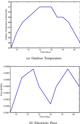
In this section, we numerically investigate the performance of the proposed satisfaction game to confirm and complement the results presented in the previous sections. Consider a building divided into three independent zones for the task of temperature control based on occupancy. The occupancy schedule of the building for a 12 hour period is shown in Figure 1. In this figure, shaded blocks indicate the time slots during which the corresponding zones in the building are occupied and needed to be conditioned. For the occupied time slots, the lower and upper bound for indoor temperature for all zones are taken to be67F and79F, respectively. The outdoor temperature and market price are depicted in Figure 2(a) and Figure 2(b), respectively according to data in [16].
Other simulation parameters are set as = 0.7, λ = 0.9, K = 15, c1 = c2 = c3 = 1, B = 100 and Lr=1.5 KW.
The energy consumption of the HVAC units is assumed to be chosen from the set {0,0.2,0.4} for both games. First, we compare the payoff of our proposed game in the satisfaction form with its payoff in the normal form and the payoff of the maximum social welfare solution as shown in Figure 3. The learning algorithm parameter is set at α= 0.05and the number of iteration is10000. The proposed learning algorithm is able to meet the optimal solution for most of the time (stochastically stable state). For the game in normal form, players can achieve NE after a few iterations, and the payoff of players is considerably lower than the maximum spacial welfare.
Figure 4 studies the effect of exploration rate (α) on the convergence of the game’s payoff in satisfaction form to the maximum social welfare. As the figure shows, by decreasing the exploration rate from 0.05 to 0.01, the players tend to stick to their choices. Therefore, the learning algorithm might temporary stabilize at a non-optimal state. On the the other hand by increasing the exploration rate from 0.05 to 0.09, the payoff decreases again. This can be explained since for higher exploration rates, players choose their actions more dynamically, and consequently the algorithm might not be
0 0.01 0.02 0.03 0.04 0.05 0.06 0.07 0.08 0.09 0.1
50 55 60 65 70 75 80 85 90
Exploration Rate (α)
Percentage of Converagence to The Optimal Solution
Fig. 4. Satisfaction game convergence versus the exploration rate
73 73.5 74 74.5
5 5.5 6 6.5 7 7.5 8 8.5 9 9.5
10x 10 −3
Average Indoor Temeparture (Fahrenheit)
Payoff
Real−Time SE
SE
Real−Time NE
NE
Fig. 5. The payoff versus the average indoor temperature
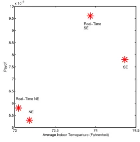
stable even if it has converged to the maximum social welfare. Next we compare the average conditioned indoor temper-ature during the scheduled time slots for zone 1 versus the achieved payoff for the four cases of day-ahead SE, day-ahead NE, real-time SE and real-time NE in Figure 5. Note that the payoff function for 12-hour cases are different from that for the real-time cases. However, the payoff achieved by the game in satisfaction form is higher than that of the game in normal form at the cost of higher average indoor temperature.
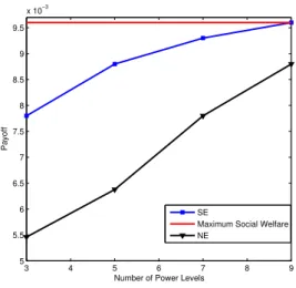
Finally, Figure 6 shows by increasing the number of granu-larity levels of the power consumed by HVAC units, the payoff increases and finally archives the maximum social welfare solution with the continuous action set. Having9power levels, the SE has a similar payoff to the maximum social welfare solution, and significantly better payoff compared to the NE payoff.
VI. CONCLUSIONS
This paper has presented a fully decentralized solution for controlling HVAC systems in smart buildings. In par-ticular, the proposed learning algorithm is able to control
3 4 5 6 7 8 9 5
5.5 6 6.5 7 7.5 8 8.5 9 9.5
x 10−3
Number of Power Levels
Payoff
SE
Maximum Social Welfare NE
Fig. 6. Payoff versus the number of power levels
the power consumption levels of HVAC units in order to guarantee that the largest number of zones have temperatures falling within predetermined comfort ranges while incurring minimum electricity costs. Simulation results demonstrate the impact of distributed control of the HVAC system on the energy-efficiency of smart-buildings.
REFERENCES
[1] T. Weng and Y. Agarwal, “From buildings to smart buildings sensing and actuation to improve energy efficiency,” inProc. of IEEE Design & Test, Special Issue on Green Buildings, vol. 29, pp. 36-44, San Diego, CA, Aug. 2012.
[2] Z. J. Liu, W. H. Qi, Z. Jia, and P. Huang, “System integration control of HVAC in intelligent building”, inProc. of Conference on Machine Learning and Cybernetics, vol. 2, pp. 1125-1128, Shanghai, China, Aug. 2004.
[3] H. Merz, T. Hansemann, and C. Huebner,Building automation commu-nication systems with EIB/KNX, LON and BACnet, Springer, Germany, 2009.
[4] M. Zaheer-uddin and G. R. Zheng, “Optimal control of time-scheduled heating, ventilating and air conditioning processes in buildings,”Journal of Energy Conversion & Management, vol. 41, no. 1, pp. 49-60, Jan. 2000.
[5] W. Shengwei and Z. Ling, “Dynamic and real-time simulation of BMS and airconditioning system as a living environment for learn-ing/training,” Journal of Automation in Construction, vol. 10, no. 4, pp. 487-505, May 2001.
[6] E. H. Mathews, D. C. Arndt, and M. F. Geyser, “Reducing the energy consumption of a conference centre - A case study using software”,
Journal of Building and Environment, vol. 37, no. 4, pp. 437-444, Apr. 2002.
[7] V. Erickson and A. Cerpa, “Occupancy based demand response HVAC control action,” in Proc. of the 2nd ACM Workshop on Embedded Sensing Systems for Energy-Efficiency in Building (BuildSys 2010), pp 7-10, Switzerland, Nov., 2010.
[8] S. Wang and Z. Ma, “Supervisory and optimal control of building HVAC systems: A review,”HVAC&R Research, vol. 14, no. 1, pp. 3-32, Jan. 2008.
[9] S. M. Perlaza, H. Tembine, S. Lasaulce, and M. Debbah, “Quality of service provisioning in decentralized networks: A satisfaction equilib-rium approach,”IEEE Journal of Selected Topics in Signal Processing, vol. 6, no. 2, pp. 104-116, Feb. 2012.
[10] J. R. Marden, H. P. Young, and L.Y. Pao, “Achieving Pareto optimality through distributed learning,” Discussion Paper, University of Colorado and University of Oxford, 2011.
[11] M. Farsi, A. Fetz, and M. Filippini, “Economies of scale and scope in multi-utilities,”Energy Journal, vol. 29, no. 4, pp. 123144, Sep. 2008. [12] J. Kwoka, “Electric power distribution: economies of scale, mergers and
restructuring,”Applied Economics, vol. 37, no. 20, pp. 2373 - 2386, Nov. 2005.
[13] P. Constantopoulos, F. C. Schweppe, and R. C. Larson, “ESTIA: A Real-Time Consumer Control Scheme for Space Conditioning Usage under Spot Electricity Pricing,”Computers and Operations Research, vol. 8, no. 18, pp. 751-765, Jul. 1991.
[14] J. F. Nash, “Equilibrium points in n-person games,”Proceedings of The National Academy of Sciences of the United States of America, vol. 36, no. 1, pp. 48-49, 1950.
[15] L. Rose, S. M. Perlaza, C. L. Martret, and M. Debbah,“Achieving Pareto optimal equilibria in energy efficient clustered ad hoc networks,” in
Proc. of the IEEE Intl. Conference on Communications (ICC), Budapest, Hungary, Jun., 2013.