Proceedings of the
Fourth International Workshop on
Graph-Based Tools
(GraBaTs 2010)
Distributed Graph-Based State Space Generation
Stefan Blom, Gijs Kant and Arend Rensink
12 pages
Guest Editors: Juan de Lara, Daniel Varro
Managing Editors: Tiziana Margaria, Julia Padberg, Gabriele Taentzer
Distributed Graph-Based State Space Generation
Stefan Blom,∗Gijs Kant†and Arend Rensink‡
[email protected] [email protected] [email protected]
Department of Computer Science University of Twente, The Netherlands
Abstract: LTSMIN provides a framework in which state space generation can be distributed easily over many cores on a single compute node, as well as over multiple compute nodes. The tool works on the basis of a vector representation of the states; the individual cores are assigned the task of computing all successors of states that are sent to them. In this paper we show how this framework can be applied in the case where states are essentially graphs interpreted up to isomorphism, such as the ones we have been studying forGROOVE. This involves developing a suitable vector representation for a canonical form of those graphs. The canonical forms are computed using a third tool calledBLISS. We combined the three tools to form a system for distributed state space generation based on graph grammars.
We show that the time performance of the resulting system scales well (i.e., close to linear) with the number of cores. We also report surprising statistics on the memory consumption, which imply that the vector representation used to store graphs in LTSMINis more compact than the representation used inGROOVE.
Keywords:Graph Transformation, Symmetry Reduction, State Space Generation, Distributed Computing,GROOVE, LTSMIN
1
Introduction
For the last two years, the development in modern computer processors has been to put more cores on a single processor, rather than to speed up individual cores. To benefit from this development, it is therefore important to find ways to utilise the power of parallel processing. So far, there is no general way to achieve this for arbitrary applications.
In the context of graph transformation, this topic has been investigated by Bergmann et al. in [BRV09] for the toolVIATRA2. The core functionality ofVIATRA2 is to compute a sequence of transformations, controlled by a predefined set of rules, as fast as possible. The paper proposes parallellisation of the matching algorithm.
In this paper, we address parallellisation ofGROOVE[Ren04], which differs from other graph transformation tools in that it aims atcomplete state space explorationfor a given set of rules, rather than computing a single sequence — where a state equates to a graph. One of the most important aspects ofGROOVE, furthermore, is that states are comparedmodulo isomorphism; that
∗Stefan Blom is partially sponsored by the EU under grant number FP6-NEST STREP 043235 (EC-MOAN).
†Gijs Kant is sponsored by the NWO under grant number 612.000.937 (VOCHS).
is, two graphs are considered to represent the same state if they are isomorphic. Though checking graph isomorphism is thought to be non-polynomial, the resulting reduction in state space size can more than make up for the cost of isomorphism checking; see, e.g., [CPR08].
At the core of our solution lies LTSMIN[BPW10], an existing framework specifically designed to enable distributed state space exploration with support for multiple specification languages. To use LTSMIN, an application has to:
1. Provide a serialisation of states in the form of fixed-lengthstate vectors. State vectors are minimised to so-calledindex vectors(see [BLPW08]), which can be efficiently stored and transmitted.
2. Be able to generate all successors of a given source state, where both the source state and the successor states are communicated in the form of such a state vector.
LTSMIN will then run parallel copies of this application on every available core; the copies communicate using message passing, so that this works equally well with parallel and distributed cores. This method of parallellisation is particularly promising forGROOVEbecause the time-intensive step of isomorphism checking is done concurrently for many states.
In the case ofGROOVE, Step 2 is present by default, but Step 1 is challenging. It is not enough to “flatten” graphs to a vector representation of some kind: in order to reduce the state space up to graph isomorphism, we have to make sure that the representative vector is the same for isomorphic graphs. For this purpose, we can make use of an existing tool calledBLISS[JK07], which computescanonical graphsbased on the principles developed in [McK81]. The LTSMIN vector representing a graph is thus the “flattening” of its canonical form.
We have experimented with this combination of LTSMIN,GROOVEandBLISS. In this paper we report two results:
• For larger cases, the time performance of the parallellised system scales well (though not linearly) with the number of processors. On a single core the setup is a good deal less efficient thanGROOVE, but a system with eight or more cores easily outperforms the stand-alone version ofGROOVE.
• Given a good vectorisation of the canonical form, the memory performance of the combina-tion of LTSMIN,GROOVEandBLISSis also a good deal better than that of the stand-alone version. This is surprising given the fact that, in contrast toGROOVE, the data structures that LTSMINuses in its tree compression and central state store are not at all optimised towards the storage of graphs. The gain is large enough to make us consider moving to the compressed vector representation even in the stand-alone, sequential version.
We introduce GROOVE in Section 2 and the relevant features of the LTSMIN framework in Section3, especially the canonical graph vector representation. In Section4we report and analyze the outcome of the experiments. Section5draws conclusions and discusses future work.
2
Graph-based state space generation
moreover, nodes are drawn either from a set of node identitiesNode, or from the set of primitive data valuesVal=Bool∪Int∪Real∪String.
Definition 1(graph, isomorphism) A graphGis a tuple hV,Ei whereV ⊆Node is a finite set of nodes andE ⊆V×Lab×(V∪Val)is a finite set of edges. We use src(e), tgt(e)and lab(e) to denoted the source, target and label of an edge e. The set of all graphs is denoted
Graph. GraphsG,Hareisomorphic, denotedG=∼H, if there exists a bijection f:VG→VH such that(f(v),a,f¯(w))∈EHif and only if(v,a,w)∈EG, where ¯f= f∪idVal. We sometimes write
f(G) =H.
There is no need to precisely define rules; we merely formalise their actions upon graphs. A rule is an objectrthat can be applied to ahost graph Gif there exists a so-calledmatch mforrin G(not formalised here, either). The rule and the match together determine a transformation ofG, formally expressed by a derivation relationG−r−,→m H, whereHis called thetarget graph. This derivation relation is well-defined and deterministic modulo isomorphism:
• G−r−,→m HandG0∼=GimpliesG0−r−,→m H0for someH0∼=H.
• G−r−,→m H1andG−r−,→m H2impliesH1∼=H2.
Using these concepts we define the graph transition system generated by a set of rules.
Definition 2(graph transition system) The graph transition system (GTS) for a set of rulesR and a start graphSis given byhQ,→,Si, where→is the derivation relation restricted toQ, andQ is the smallest set of graphs such that (i)S∈Q, and (ii)H∈Qfor allG∈Q,r∈RandG−r−,→m H.
The GTS is a labelled transition system as used in many verification methods, in particular model checking [BK09]. Unfortunately, the GTS can easily be infinite, and even when finite can grow extremely large even for small start graphs — a phenomenon calledstate space explosion. One way to combat state space explosion is throughsymmetry reduction(see, e.g., [CJEF96]). In the case of graphs, symmetries show up as isomorphisms; the state space can be reduced by collapsing all isomorphic states, or in other words, taking the quotient of the GTS under∼=. The following algorithm generates this quotienthQ,T,Si(whereT is the set of transitions).
1 let Q:={S}, T:=/0, F:={S} (Fis the collection of fresh states) 2 while F6=/0
3 do choose G∈F (whichGis chosen depends on the structure ofF) 4 let F:=F\ {G}
5 for G−r−,→m H
6 do if ∃H0∈Q:H0∼=H
7 then let H:=H0
8 else let Q:=Q∪ {H}, F:=F∪ {H}
9 endif
10 let T :=T∪ {(G,r,m,H)}
11 endfor
The crux is in Line6, which tests formembership up to isomorphism: given a graphHand a set of graphsQ, findH0∈Qsuch thatH0∼=H. TestingH0∼=Hfor given graphsH,H0is believed to be non-polynomial in|H|(see [Wei02]), and clearly membership up to isomorphism generalises the pairwise test. However, we have shown in [Ren07,CPR08] that the gain by symmetry reduction can be huge, and hence can be worthwhile despite its complexity. We now discuss two ways to implement membership modulo isomorphism.
Graph certificates. The current implementation of GROOVE, as reported in [Ren07], uses certificatesto obtain a data structure forQallowing a membership-up-to-isomorphism test that performs well in many practical cases.
Anode certifieris a functionnc:Graph→Node*Nat, which for every graphGresults in a function ncG:VG→Nat with the property thatncG=ncH◦f for all isomorphisms f from Gto H. Agraph certifier is a function gc: Graph→Nat such that G∼=H impliesgc(G) =
gc(H). An easy example of a node certifier is to count the number of incident edges (ncG:v7→
|{e∈EG|src(e) =v∨tgt(e) =v}|for allv∈VG). Every node certifierncgives rise to a graph certifiergc:G7→∑v∈VGnc(v).
GROOVEcurrently implementsQas a mapNat→2Graphsuch thatn7→ {G∈Q|n=gc(G)}. FindingH0∈Qsuch thatH0=∼Hcomes down to searchingQ(gc(H)), which for a good graph certifiergcis almost always either empty or a singleton set. Moreover, pairwise testingH0∼=H for theH0∈Q(gc(H))is made easier by using a node certifier.
Canonical forms. One can take the idea of graph certifiers one step further by also requiring thatgc(G) =gc(H)impliesG∼=H. This is the idea behind the concept ofcanonical forms.
Agraph canoniseris a functioncan:Graph→Node*Node, which for every graphGresults in an injective functioncanG:VG→Nodesuch thatG∼=Hif and only ifcanG(G) =canH(H). (Note that, in combination with a hash functionhash:Node→Nat, this gives rise to a node certifiernc=hash◦can.)Qcan then be implemented as a set of canonical form graphs. Obviously, computing canonical forms is as complex as testing for isomorphism; nevertheless, in practice the complexity often turns out to be bearable. In particular, the algorithm developed by McKay [McK81] as implemented in the toolsNAUTY[McK09] andBLISS[JK07] does well in practice. We have usedBLISSin our experimentation in the distributed setting. There is a discrepancy in thatBLISSuses node-labelled rather than edge-labelled graphs; however, our graphs can be converted toBLISSgraphs without loss of information, though with a slight blowup due to the need to encode edge labels in some way. Another noteworthy property is that the canonical forms produced byBLISSalways map to an initial fragment ofNat; that is,canG(VG) ={0, . . . ,|VG| −1} for all graphsG. BLISSreorders the nodes such that for isomorphic graphsGandHfor allv∈G the same number is assigned tovand f(v)∈Hfor some isomorphism f (withH= f(G)).
3
The LTS
MINframework
B
L
IS
S
G
R
O
O
V
E
B
L
IS
S
G
R
O
O
V
E
B
L
IS
S
G
R
O
O
V
E
LTSMIN LTSMIN LTSMIN
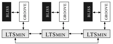
Figure 1: 3-core configuration of LTSMINwithGROOVE+BLISSas user module.
calledPINS, forPartitioned Next-State function. We will briefly explain the underlying concepts. To run an application on top of the LTSMINframework, an LTSMINclient as well as a copy of the user module is started up in parallel on every core. These copies communicate by message passing, so that it does not matter (from the protocol view) whether cores are on a single machine or distributed over different machines. State space exploration then proceeds as follows:
• LTSMINdefines a function that associates a fixed core with each state, on the basis of the state’s vector representation. When a state is generated, it is sent to the associated core for further processing. The exploration is kicked off by sending the initial state to the appropriate core.
• Each core keeps a store of all states sent to it so far, remembering also whether the states are closed (i.e., already fully explored) or fresh.
• Upon reception of a state, a core adds it to its state store, marking it as fresh if it was not already in the store.
• Each core computes the successor of each fresh state, and sends the successors to their associated cores. This computation is done by the user module.
An example configuration withGROOVEandBLISSis depicted schematically in Figure1.
3.1 State vectors and tree compression
The central concept enabling the modularity of LTSMINis thestate vector. Every state has to be presented as a vectorhp1, . . . ,pnifor fixedn. The nature of the elementspiactually does not matter, as these are immediately mapped to table indices for each position. That is, fori=1, . . . ,n LTSMINbuilds up an injective mappingti:Pi→Nat, wherePiis the set of all values encountered so far at positioniandNat is a finite fragment of natural numbers; e.g., that fragment which can be represented in 32 bits. Every state vectorhp1, . . . ,pniis then converted to anindex vector
ht1(p1), . . . ,tn(pn)i ∈Natn. The mappingsti are generated on the fly: once a value is encountered for the first time (on positioni) it is added toti; from then on the same value on that position will always be mapped to the same index. The function associating a core with each state is computed as a hash on the index vector, modulo the number of available cores.
The tables (ti)1≤i≤n, together called the leaf database, are duplicated in the system. It is
known on the side of the user module, since this is where the coding of state vectors to and from index vectors actually takes place. Thus, in a system withccores, alltiare replicated 2ctimes.1
Index vectors are further compressed using so-calledtree compression(see [BLPW08]): with-out going into details, this comes down to repeatedly grouping neighbouring positions of the index vector and building a new table of all combinations of values at those positions that are found during exploration. All these tables together form what is called thetree database.
The success of the method crucially depends on finding a state vector representation that has as few values at each vector position as possible; i.e., each of thePishould be small. This does not contradict a huge overall state space size: for maxi|Pi|=m, the number of states that can potentially be represented ismn. In the worst case, for one or morei|Pi|approaches the total state space size, and hence so does the size of the tree database; the advantage of this compression method is then completely lost.
3.2 Serialising canonical form graphs
We will now describe the steps necessary to use GROOVEas a user module in the LTSMIN framework. The main difficulty is to find a suitable state vector representation. This is entirely up to the user module: LTSMINgets to see the state vectors only after they have been produced, and treats the values in thePias completely unstructured.
It is absolutely necessary that the state vectors uniquely represent states. This means that, if we want to benefit from symmetry reduction, we have to put graphs into canonical formbefore communicating them to LTSMIN. Moreover, as explained above, the vector representation should ideally have only few possible values at each slot.
In Section2we have explained that the canonical form computed byBLISSessentially assigns a sequence number from 0 to|V| −1 to each node of a graphG. This imposes a total ordering≤
onV; we will use~v=v0· · ·vk to denote the ordered sequence of nodes inV. Furthermore, we use the natural total orders on the primitive valuesInt,String,BoolandRealand we assume a total order onLab(for instance, the alphabetical ordering). This also gives rise to a lexicographical ordering on edges. In the sequel,ord(X)for a setX with an implicit order will denote the ordered vector ofX-elements, and~xI for a sequencex∈X∗ and an index setI⊆ {0, . . . ,|~x| −1}will denote the sequence of elements at positionsI.
The vector~pGrepresentingGwill consist ofnslots, of which the first contains a sequence of node colours(i.e., the primitive value in the case of value nodes or the set of self-edges for the other nodes; this is also used in the conversion to coloured graphs, needed for the use ofBLISS), one for each node, in the order imposed by the canonical form; the second to fifth contain the sets of primitive values fromValused as target nodes, seperated per primitive type; and the remaining slots contain outgoing edges for the individual nodes. Ifk>n−5 (wherek=|VG|andn=|~p|) then nodes are “wrapped around”, e.g. forn=12 slotp5would be used forv0,v7,v14, . . .. This
way graphs can be encoded into a fixed size vector, even if the size of the graphs is not fixed.
1This description is actually still slightly simplified with respect to the implementation: there the encoding of the
outgoingstates may be different from that of theincomingones; the former is then local to each core, and the LTSMIN
-10 B
”hi”
A
A 3
a i
i
b
n i a
0
1
2 3
4
5
p0={A} {A} {B}(Int,1) (Int,0) (String,0) list of nodes
p1=−10 3 list ofInts
p2=“hi” list ofStrings
p3=ε (the empty sequence) list ofBools
p4=ε list ofReals
p5={(a,2),(b,1),(i,3)} /0 edges of0and4 p6={(a,2),(i,3)} /0 edges of1and5
p7={(i,4),(n,5)} edges of2
p8=/0 edges of3
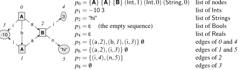
Figure 2: An example graph with |V|=6, represented by a state vector with |~p|=9. The canonical node numbers are in italic. Node labelsA,Bare self-edges; oval nodes are data values.
Formally this is defined by
pi=
colorG(v0)· · ·colorG(vk) ifi=0
XG ifi=1+jandX= (Int String Bool Real)j outG(w0)· · ·outG(wm) ifi=5+jand~w=~v{l|l= jmod(n−5)}
wherecolorG(v)denotes the colour andoutG(v)the outgoing edges ofv, defined as follows:
colorG(v) =
selfG(v) ifv∈Node
(X,i) ifv=XGi,
selfG(v) ={a|(v,a,v)∈EG},
XG=ord(X∩tgt(EG)) forX=Int,String,Bool,Real, outG(v) ={(a,canG(w))|(v,a,w)∈EG,v6=w}.
An example state vector is shown in Figure2. As related above, this is translated to an index vector together with a set of tablest0, . . . ,tn, so that a value at positioniwhich recurs in another
state vector at the same position is encoded by the same index. For instance, if the graph in Figure2is modified byi:=3 in node 0, only slot 5 of the state and index vectors would change (namely to{(a,2),(b,1),(i,4)}/0) and onlyt5might have to be updated with this new value.
4
The experiments
We have carried out experiments based on three rule systems with varying characteristics.
le A leader election protocol. In this case there is a fixed number of nodes representing network nodes and a varying number of nodes representing messages. The number of nodes is an upper limit on the number of messages. This case study has been used for the GraBaTs 2009 tool contest (seehttp://is.tm.tue.nl/staff/pvgorp/events/grabats2009).
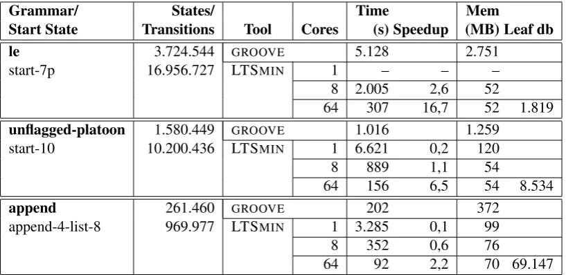
Table 1: Results for the largest start graphs where bothGROOVE(sequential) and LTSMIN(1, 8 and 64 cores) were able to generate the state-space. The memory usage shown is the average per core. The last column shows the number of elements in the global leaf database for LTSMIN.
Grammar/ States/ Time Mem
Start State Transitions Tool Cores (s) Speedup (MB) Leaf db
le 3.724.544 GROOVE 5.128 2.751
start-7p 16.956.727 LTSMIN 1 – – –
8 2.005 2,6 52
64 307 16,7 52 1.819
unflagged-platoon 1.580.449 GROOVE 1.016 1.259
start-10 10.200.436 LTSMIN 1 6.621 0,2 120
8 889 1,1 54
64 156 6,5 54 8.534
append 261.460 GROOVE 202 372
append-4-list-8 969.977 LTSMIN 1 3.285 0,1 99
8 352 0,6 76
64 92 2,2 70 69.147
append A model of list appenders that concurrently add a value to the same list. In this case the number of nodes grows in each step. The maximal number of nodes equals the number of appenders plus 1 times the number of elements in the list. There is hardly any nontrivial isomorphism in the transition system.
The experiments have been performed on a cluster consisting of 8 compute nodes with 4 dual Intel E5520 CPUs each and 24GB RAM, for a total of 8 cores per compute node and 64 cores in total.GROOVE4.0.1 has been used with a Sun Java 1.6.0 64-bit VM with a maximum of 2GB of memory for each core. For computing canonical forms we usedBLISS0.50. We used LTSMIN1.5, with an added dataflow module to facilitate the communication between LTSMINandGROOVE. For all experiments, the combined system was given a time limit of 4 hours. The state vector size for the first two cases was chosen such thatn≥k+5, hence no slot needs to encode the edges of more than one node; however, this is not the case for the third case.
We have compared the performance of the distributed setting with the default, sequential implementation of GROOVE(without computation of canonical forms), running on the same machine but with a memory upper bound of 20GB. For the leader election with start state start-7pa different machine with 60GB of memory has been used, because with 20GB of memory the result could not be calculated.
Where there are no values in the table or figures of this section, either the time limit of 4 hours was exceeded or there was not enough memory.
increase from 1 to 8 cores and from 8 to 64 cores is sizeable, though below the optimal value of 8. Furthermore, the leaf database of the append rule system grows much larger than for the others, despite the fact that the state space is much smaller. This is a consequence of the fact that the graph size outgrows the vector size for this case.
101 102 103 104 105 106 107 108 109 start-03start-04start-05start-06start-07start-08start-09start-10start-11start-12 states transitions leaf db
(a) Number of states, transitions and leaf values.
1 10 100 1000 10000
start-03start-04start-05start-06start-07start-08start-09start-10start-11start-12start-13
Memory (MB)
groove 1 8 64
(b) Memory usage forGROOVEand LTSMIN(per core).
0.1 1 10 100 1000 10000 100000
start-03start-04start-05start-06start-07start-08start-09start-10start-11start-12start-13
Time (s) groove 1 8 16 32 64
(c) Execution time.
0 1 2 3 4 5 6 7
start-03 start-04 start-05 start-06 start-07 start-08 start-09 start-10
Speedup groove 1 8 16 32 64
(d) Speedup compared toGROOVE.
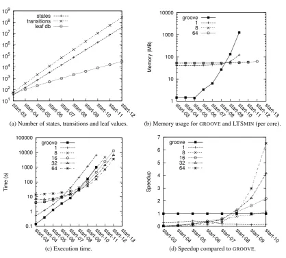
Figure 3: Figures for the car platooning case for different start states.
Time and memory distributions. For the car platooning case, more detailed results are shown in Figures3and4. First of all, Figure2ashows that even though the size of the problem grows exponentially, the number of elements of the leaf value database of LTSMINdoes not. This is also reflected by the per-core memory usage of LTSMIN(Figure2b), which seems hardly to grow, in contrast to the more than exponentially growing memory usage ofGROOVE.
0 5 10 15 20 25 30 35 40 45
groove8 16 24 32 40 48 56 64
Time (s)
iso enc/dec send/recv
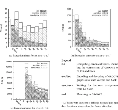
(a) Execution times forstart-08.∗
0 200 400 600 800 1000 1200
groove8 16 24 32 40 48 56 64
Time (s)
iso enc/dec send/recv
(b) Execution times forstart-10.∗
0 2000 4000 6000 8000 10000 12000 14000
groove1 8 16 24 32 40 48 56 64
Time (s)
iso enc/dec send/recv
(c) Execution times forstart-12.
Legend
iso Computing canonical forms, includ-ing the conversion of GROOVE to
BLISSand back
enc/dec Encoding and decoding ofGROOVE
graphs into state vectors and back
send/recv Waiting for the next assignment from LTSMIN
rest Matching inGROOVE
∗LTSMINwith one core is left out, because it is more
then five times slower than the fastest after that.
Figure 4: Decomposed execution times for the car platooning case for different numbers of cores.
Execution time decomposition. Figure4shows how the execution time is built up. For smaller start states, the communication between cores (labelled “send/recv” in the figure) is a major factor in the computation time for LTSMIN, but for larger start states most of the time is spent on computing canonical forms (isomorphism reduction). As the number of cores grows, however, the communication again starts to play a larger relative rule — which is to be expected since this is the only task that isnotparallellised; indeed, the communication overhead grows more than linearly with the number of cores.
Analysis. For lack of space we cannot include all results in this paper, but the trends for the leader election and append rule systems are very similar to the ones reported above for car platooning. Based on these results, we come to the following observations:
Although the canonical form calculation can renumber nodes in an unpredictable manner, which in the worst case could blow up the number of leaf values, apparently the different states are really a combinatorial result of the different parts of the vector. This is especially true for the leader election and car platooning cases, where the number of nodes is a priori bounded and the vector size can be chosen to accomodate this; in the append case, where the state vector representation has to reuse slots for multiple nodes, the results are less spectacular, though still quite good.
• The memory performance of the distributed LTSMINsolution is better than that of the sequentialGROOVEsystem. This is a direct consequence of the success of the serialisation, but it deserves a separate mention. GROOVEuses dedicated data structures, which store only the difference (delta) between successive graphs; nevertheless, the very general tree compression algorithm of LTSMINturns out to beat this hands down. This came as a big surprise to us, and is reason to reconsider the data structures ofGROOVE.
• The time performance of the distributed LTSMINsolution scales well with the number of cores, especially for larger start graphs. The performance of a single core is quite bad compared toGROOVE, taking in the order of 8-10 times as much time, but the distributed system with 8 or more cores is faster. For the largest cases thatGROOVEstill can compute, we get speedups up to 16 (for 64 cores); moreover, the LTSMINsolution continues to scale well for larger start graphs, whichGROOVEon its own cannot cope with at all any more.
• The canonical form computation in the LTSMIN-based system lasts as much as 5 times longer than isomorphism checking in stand-aloneGROOVE. As the certificate-based solution ofGROOVEuses the same underlying technique asBLISS’ canonical form computation (namely, repeated partition refinement), there is no obvious reason for this performance penalty; we hypothesize that it is a consequence of the required encoding of edge-labelled GROOVEgraphs as node-labelledBLISSgraphs, which increases the graph size. It therefore seems interesting to reimplement theBLISSalgorithm for edge-labelled graphs. Given the fact that isomorphism checking is a major fraction of the total time, we expect that this may further improve the distributed performance.
5
Conclusion
We showed a successful way of parallellising graph-based state space generation, using a combi-nation of three tools:GROOVE,BLISSand LTSMIN. A nontrivial step is the encoding of arbitrary graphs into fixed-sized state vectors. We concluded that the resulting system scales well with the number of cores, and has a surprisingly good memory performance — so good, in fact, that it might be worth replacing the currentGROOVEdata structures. We also observed that a further performance gain can probably be made by reimplementing the functionality ofBLISSin order to take advantage of the structure of edge-labelled graphs.
This in turn would allow more of the functionality of LTSMINto be used, namely the symbolic storage of states. Though there are examples where symmetry reduction has a huge payoff, the same is true, to an even larger degree, for symbolic representations. This is a subject for future investigation.
Bibliography
[BK09] C. Baier, J.-P. Katoen.Principles of Model Checking. MIT Press, 2009.
[BLPW08] S. C. C. Blom, B. Lisser, J. C. van de Pol, M. Weber. A Database Approach to Distributed State Space Generation. In Cern´a and Haverkort (eds.), Parallel and Distributed Methods in verifiCation (PDMC). Electr. Notes Theor. Comput. Sci. 198, pp. 17–32. Elsevier, 2008.
[BPW10] S. C. C. Blom, J. C. van de Pol, M. Weber. LTSMIN: Distributed and Symbolic Reachability. InComputer-Aided Verification (CAV). LNCS 6174. Springer, 2010. Seehttp://fmt.cs.utwente.nl/tools/ltsmin/.
[BRV09] G. Bergmann, I. R´ath, D. Varr´o. Parallelization of Graph Transformation Based on Incremental Pattern Matching. In Boronat and Heckel (eds.),Graph Transformation
and Visual Modeling Techniques (GT-VMT). Electr. Comm. of the EASST 18. 2009.
[CJEF96] E. M. Clarke, S. Jha, R. Enders, T. Filkorn. Exploiting Symmetry in Temporal Logic Model Checking.Formal Methods in System Design9(1/2):77–104, 1996.
[CPR08] P. Crouzen, J. C. van de Pol, A. Rensink. Applying Formal Methods to Gossiping Networks with mCRL and Groove.ACM SIGMETRICS Performance Evaluation
Review36(3):7–16, December 2008.
[JK07] T. Junttila, P. Kaski. Engineering an efficient canonical labeling tool for large and sparse graphs. In9th Workshop on Algorithm Engineering and Experiments. Pp. 135– 149. SIAM, 2007. Seehttp://www.tcs.hut.fi/Software/bliss/.
[McK81] B. D. McKay. Practical graph isomorphism.Congressus Numerantium30:45–87, 1981.
[McK09] B. D. McKay.NAUTYUser’s Guide (Version 2.4). Nov. 2009. Seehttp://cs.anu.edu. au/∼bdm/nauty/nug.pdf.
[Ren04] A. Rensink. TheGROOVESimulator: A Tool for State Space Generation. In Pfaltz et al. (eds.),Applications of Graph Transformations with Industrial Relevance (AGTIVE). LNCS 3062, pp. 479–485. Springer Verlag, 2004.
[Ren07] A. Rensink. Isomorphism Checking inGROOVE. In Z¨undorf and Varr´o (eds.),
Graph-Based Tools (GraBaTs). Electr. Comm. of the EASST 1. September 2007.
[Wei02] E. W. Weisstein. Isomorphic Graphs. From MathWorld – A Wolfram Web Resource.