Selected Revised Papers from the
4th International Workshop on
Graph Computation Models
(GCM 2012)
XL4C4D – Adding the Graph Transformation Language XL to
CINEMA 4D
Ole Kniemeyer and Winfried Kurth
10 pages
Guest Editors: Rachid Echahed, Annegret Habel, Mohamed Mosbah Managing Editors: Tiziana Margaria, Julia Padberg, Gabriele Taentzer
XL4C4D – Adding the Graph Transformation Language XL to
CINEMA 4D
Ole Kniemeyer1and Winfried Kurth2
MAXON Computer GmbH, Max-Planck-Str. 20, 61381 Friedrichsdorf, Germany
Georg-August-University G¨ottingen, Department of Ecoinformatics, Biometrics and Forest Growth, B¨usgenweg 4, 37077 G¨ottingen, Germany
Abstract: A plug-in for the 3D modeling application CINEMA 4D is presented which allows to use the graph transformation language XL to transform the 3D scene graph of CINEMA 4D. XL extends Java by graph query and rewrite facilities via a data model interface, the default rewrite mechanism is that of relational growth grammars which are based on parallel single-pushout derivations. We illustrate the plug-in at several examples, some of which make use of advanced 3D features.
Keywords:Scene graph, L-system, relational growth grammar, CINEMA 4D
1
Introduction
Most 3D modeling systems represent their 3D content as a scene graph. In general, this is a directed acyclic graph or even just a tree, where nodes contain geometry data and further properties, while edges define spatial and logical relations between nodes. E.g., the coordinate system of a node is typically inherited to its children, and often this also holds for properties like the color.
To create and modify the scene graph, 3D modeling applications typically do not only provide direct user interaction, but also built-in (textual or visual) programming languages. But none of these languages makes use of graph transformation techniques, although they suggest themselves for such a language, given the underlying scene graph.
What has been used for 3D scene graph creation are L(indenmayer)-systems [PL90], starting with the successful specification of 3D plant models, and nowadays this parallel string-rewriting formalism is directly supported by many 3D modeling applications. But as it is based on strings, it necessitates an additional interpretation step from strings to graphs. In previous research, we developed relational growth grammars as a rewriting mechanism for graphs which incorporates both the possibilities and ease of use of L-systems (but applied to graphs) and of true graph transformations based on single-pushout derivations [KBHK08,Kni09].
plant modeling in mind, so it provides strong support for this field of application, while it has fewer general 3D features than traditional all-purpose 3D modeling systems.
Through the data model interface of XL, it is possible to let XL operate on any kind of graph. We will present an implementation for the scene graph of CINEMA 4D [MAX] as a plug-in, and we will show some examples of its application.
2
Relational Growth Grammars
In this section, we will sketchrelational growth grammars(RGG for short) to have a formal basis for the following applications. We do not give complete definitions here as this would become too lengthy, they can be found in [Kni09].
At first, thegraph modelhas to be specified. To be able to use type hierarchies known from object-oriented programming for nodes and edges, and to store attributes at nodes, we are using typed attributed graphs with inheritance [EEPT06]. Since the semantics of edges within the RGG formalism is to stand for plain relationships between their incident nodes, we exclude the possibility of edge attributes, and parallel edges of the same type are not allowed. The latter means that the edges of a graphGare simply represented as a subset ofGV×ΛE×GV, whereGV denotes the nodes ofGandΛE is the set of edge types.
The rewriting mechanism of relational growth grammars is based on the algebraic single-pushout (SPO) approach [EHK+97]. The SPO approach has the nice properties that dangling edges are removed automatically, and that deletion is prefered over preservation in case of a conflict. This is very useful for the domain of models we are interested in: E.g., think of an animal being represented as a node, then there might be a rule describing death because of ageing which simply deletes the animal node. Without the automatic deletion of dangling edges, we would have to take into account all possible edges of the animal in the death rule, which would be cumbersome in practice. If there is a second rule for the animal which models its movement, and if both rules are applied in parallel, there is a conflict between deletion and preservation, but it makes perfect sense to prefer deletion as the death rule models a deliberate and rather drastic event.
In order to instantiate the SPO approach for RGG graphs, we have to define a corresponding categoryRGGGraphof graphs and their homomorphisms. The single-pushout approach works withpartial homomorphismsHomP(G,H), i. e., graph homomorphismsG→H which are de-fined on some subgraph of their domainG. To integrate the inheritance relation in the notion of a graph homomorphism, we use a technique based on [PEM87]: A homomorphism f :G→H inRGGGraphis a structure-preserving mapping such that for every object (node or edge)x∈G the type of its image f(x)is a subtype of the type ofx.
have to either specify several productions (one for each possible number of children) or to use several derivation steps. Both solutions are not feasible from a practical point of view. The dependence of the right-hand side on the match provides a solution to this problem (cf. [Kur94,
PKL07,CJ92]). As a result, an RGG rule consists of a left-hand sideL, an application condition cand a mapping pwhich maps a matchmforLto the actual SPO production p(m)to be used for the derivation:
Definition 1(Application Condition) LetLbe a graph. Anapplication condition con the set Hom(L,·) of all total graph homomorphisms with domain L is a boolean-valued function on Hom(L,·).
Definition 2(Simple RGG Rule) LetLbe a graph. A simple RGG rule r= (L,c,p)is given by a graph L, an application condition c, and a mapping p : Hom(L,·)→ MonP(·,·), where MonP(·,·)denotes the set of all partial, injective homomorphisms, such that for somem:L→
G∈Hom(L,·) the image p(m) is an SPO production M(m)−−→p(m) R(m)whose domain (in the categorical sense)M(m)is a subgraph ofGand a supergraph ofm(L).
Definition 3(Match) Amatchfor a simple ruler= (L,c,p)in a host graphGis a total graph homomorphismm:L→Gsuch that the application conditioncis fulfilled (c(m) =true).
Definition 4(Simple RGG Derivation) Letm:L→Gbe a match for a simple ruler= (L,c,p). Adirect derivationusingrviam, denoted asG=r⇒,m H, is given by a direct SPO derivation using
M(m)−−→p(m) R(m)via the inclusionM(m),→G, i. e., by the following commutative diagram in the categoryRGGGraph, where the square is a pushout:
L
m
(
(
/
/ m(L) // M(m) p(m) //
_
R(m)
G // H
The following is an example for a simple RGG rule which moves some sort of animal (A-typed node) along a path of X-(A-typed nodes if its energy is above the threshold 1 and creates some children at the left location, the number depending on the energy.
L=
aA
xX //
O
O
yX
,c(m) = (m(a).energy>1), p(m) =m(L)→Rbm(a).energyc
withR1=
aA
xX //yX
O
O
,R2=
A aA
xX //
O
O
yX
O
O
,R3=
A A aA
xX //
O
O
`
`
yX
O
O
Nodes are represented as oval boxes around their type, node identifiers are placed before the upper left corner. m(a).energy refers to the value of the energy attribute of the match for the A-typed nodea, and bxcdenotes the integral part of x (floor function). The mapping p(m) is indicated by the reuse of node identifiers of the LHS for the RHS.
Because processes in a living system happen in parallel, there has to be the possibility to apply RGG rules in parallel. For a family of simple RGG rules with corresponding matches, we can create aparallel derivationfrom the generated SPO productionspi(mi)as defined in [EHK+97]. The following shows such a parallel RGG derivation for the single example rule from above using the two obvious matches, if we assume that the energy of nodeais 1.5 and that ofbis 3.5.
G
aA bA
X //X //
O
O
X //
O
O
X //X
+
3 H
A A
aA bA
X //X //X
X
X FF
/ / O O X O O / / X
Unfortunately, this straightforward parallelism fails if rule application successors of neigh-bouring parts shall be connected by edges, which is a very important case and needed by the embedding of L-systems in the RGG formalism. Severalconnection mechanisms were studied in [LR76] to address this problem, of which theoperator approach [Nag76,Nag79] turns out to be a suitable technique for relational growth grammars. The application of a rule to a match also establishesconnection transformationswhich are given by a quintuple(s,(A,d,γ),t)with a nodesfrom the match, a nodetfrom the right-hand side, anoperator A, a direction flagd(either “source” or “target”) and an edge typeγ. An operatorAyields for every noden∈Gof the match a setAG(n)of related nodes (e. g., its neighbours).
We may think of such a connection transformation as an arrow which points from a node s in the host graph G to a node t in the derived graph H resulting from the simple RGG derivation. The operator mechanism then shifts connections within the host graph along a pair of matching arrows to the derived graph: For a matching arrow pair (s1,(A1,“source”,γ),t1),
(s2,(A2,“target”,γ),t2)where the host graph nodess1,s2are related according to the operators,
i. e.,s2∈A1(s1) ands1∈A2(s2), an additionalγ-typed edge fromt1 tot2 is created within the
derived graphH.
Definition 5(RGG Rule) AnRGG rule r= (L,c,p,z)is a simple RGG rule(L,c,p)together with a mappingzwhich assigns to each matchm:L→Gfor the simple rule a set of connection transformations(s,(A,d,γ),t)withs∈M(m)(domain of p(m)),t∈R(m)(codomain of p(m)), an operatorA, a directiond(either “source” or “target”) and an edge typeγ.
3
The XL Programming Language
square brackets instead of the usual curly braces. The following example shows the translation of the animal movement and reproduction RGG rule from above:
[
x:X [a:A] y:X, (a.energy > 1) ==>>
x for(i n t i = 2; i <= a.energy; ++i) ( [A] ) y [a];
]
x:Xis a pattern which matches a node of Java classXand assigns the identifierxto the match. Within and right-hand sides, square brackets are used to enclose branches, so that the left-hand side of the example has to be read as: Find anX-typed nodexwhich has anA-typed child aand anX-typed successory. Child and successor relationships are represented by distinct edge types. The left-hand side also contains an application condition in round parentheses.
The right-hand side depends on the match because the for-loop expands into a variable number of nodes, depending ona.energy: If the energy is less than 2, we havex y [a]which just movesatoy. If it reaches 2, we getx [A] y [a]. This creates a newAnode (because there is no node identifierA) as a child ofx. For higher energies, we get even more newAnodes.
Cycles of non-tree-like structures are obtained by repeating a node identifier. E.g., the pattern a:A B C arepresents a circular graph of three nodes of typesA,B,C.
Graph queries are expressions which use the syntax of left-hand sides within(* *). E.g., the expressioncount((* x [A] *))contains a query for allA-typed children of a given node x, and counts the number of matches.
All graph operations of XL are defined on top of an abstract data model interface. By im-plementation of this interface, XL can operate on any kind of graph. The most sophisticated implementation exists for GroIMP, but there are also implementations for XML documents or minimalistic Sierpinski graphs [Kni09].
In the following, we will show some more examples of XL. An in-depth description can be found in [Kni09].
4
The Plug-In XL4C4D and Its Application
The 3D modeling system CINEMA 4D [MAX] uses a scene graph to represent spatial and logical relations between objects. In fact it is rather a tree than a graph, but objects can have additional link attributes which may point to arbitrary objects in the scene tree, thus yielding a true graph.
Each object has its own local 3D coordinate system. As usual for scene graphs, this is de-fined by the coordinate system of the parent object, multiplied with a transformation attribute of the object itself, so that an object moves together with its descendants when one modifies the transformation of the object. There are objects with a geometry such asCube, Sphere, or PolygonObjectfor a general polygon mesh, but also aNullobject which has no geometry itself, but can be used to group its children and to inherit its transformation to them. Instanceobjects also have no geometry themselves, but a link to another object. They show the geometry of the linked object within their own coordinate system. This saves a lot of memory when one wants to place the same geometry at several locations.
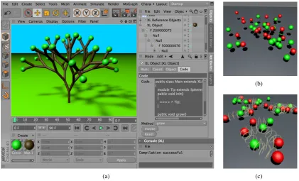
(a)
(b)
(c)
Figure 1:(a)Screenshot showing the plug-in with a binary tree;(b,c)polymerization model
interface for CINEMA 4D’s scene graph. The plug-in (available at [KHK]) adds the following features to CINEMA 4D:
• The XL Consoleshows output from XL execution, and it allows to directly type in XL code which is then executed.
• There is a new scene graph object XL Object. It has a code attribute which allows to enter a complete XL program. Methods of the program may be invoked interactively, and parameters defined in the program are accessible in the attribute manager.
• The XL Instance object behaves similar to a normal Instance object. It has additional attributes for scaling and translation which are more convenient for XL models than the normal transformation attributes.
Figure1(a) shows a screenshot of CINEMA 4D at the example of a simple 3D binary tree. The code properties of the singleXL Objectare opened. The complete code for the model is
public class Main extends XLObject {
module Tip extends Sphere(20).(setMaterial("Green"));
public void init() [ ==>> ˆ Tip; ]
public void grow()
The code shows the basic structure of an XL model within XL4C4D: The actual code has to be surrounded by a class extending XLObject. Parameterless public void methods of that class can be invoked interactively by choosing them in a drop-down menu and clicking on an Invoke-button, so one typically puts the actual rules within such methods. In the example there is aninit-method with a simple RGG rule with empty LHS: Out of nothing, the rule creates a two-node graph starting at theXL Object itself, which is represented byˆ, and followed by an instance ofTip. The Java classTip itself is specified in amoduledeclaration which is a simplified class declaration and in this case corresponds to aSphereobject in the scene graph with a radius of 20 units and the material named ”Green”.
ATip-node represents a leaf (in the mathematical sense) of the tree, therefore for a growth of a binary tree such a node has to be replaced by an inner node bearing two newTip-nodes. This is implemented by thegrow-method which uses a non-simple RGG rule to replace (in parallel) eachTip-node by anF-node with two branches. The branches do not consist ofTip-nodes only, but also of 3D rotation nodes of the typesRUandRHput in front. AnF-node corresponds to an XL Instanceobject in the scene graph which instantiates aCylinderobject, the parameter 100 to theF-constructor scales this cylinder to a height of 100 units, and it also shifts the coordinate system by 100 units along the cylinder axis (the local y-axis). Together with the rotations around the local x- and y-axes (RU andRH, respectively), this places the base of the cylinder at the location of the previous Tip, and adds the two new tips at the top of the cylinder, but with a rotated coordinate system such that the new branches emerge in different directions in 3D space. Thegrow-rule requires connection transformations (there are no common nodes on LHS and RHS for gluing). They can be specified for each pair of LHS/RHS-nodes, but for convenience two such transformations are automatically added if one uses the rule arrow==>, namely one from the leftmost (unbracketed) LHS node to the leftmost (unbracketed) RHS node and one for the rightmost nodes. This is exactly what is needed for an L-system rule when it shall be applied not to a string but to a graph.
Besides Sphere, F, RU and RH, the plug-in also provides RL for rotation around the z-axis,Mfor y-translation,Scalefor uniform scaling,Nullfor general transformations,Cube, Box, Instance, and even Springfor physics simulations. Each node of such a Java class corresponds to a CINEMA 4D object of suitable type, e.g., pure transformation nodes are rep-resented as Null objects in the scene graph. The general BaseObject class corresponds to CINEMA 4D’sBaseObjectC++ class. With its methods and the numerical IDs from CINEMA 4D’s resource files it is possible to create objects of any type, and to set most of their attributes. Attributes of the CINEMA 4D typesBool,LONG,Real,Vector,Matrix,StringandBaseLinkare supported, the same holds for additional user data attributes.
One of CINEMA 4D’s advanced features is the Dynamics module which provides a rigid body simulation. With its help we can create a toy model of polymerization: A lot of monomers of two types (MonomerAandMonomerB) move around according to the laws of rigid body physics. At each frame (i.e., each simulation step), it is checked if two monomers of different type come close to each other. If so, the rule triggers and creates a bond in the form of aSpringobject for the rigid body simulation:
public class Main extends XLObject {
module MonomerB extends Sphere(20).(setColor(0, 1, 0));
public void init() [ ... ]
public void step()
[
a:MonomerA, b:MonomerB,
((distance(a, b) <= 50) && empty((* Spring(a, b) *)))
==>> a, b, ˆ Spring(a, b).(setBoolean(FORCE_ALWAYS_VISIBLE, true)); ]
}
The bonding rulesteplooks for two monomersa,bwhich, due to the comma inbetween, need not have any relationship in the graph. Its application condition tests ifa, bare close to each other (at most 50 units in 3D space) and makes sure by a graph query that noSpring node already exists. The RHS repeatsa,bso that they don’t get deleted, and it creates and initializes a newSpringnode linked to them.
The setup of the simulation environment for the example is done manually. Figure1(b)shows the initial situation with monomers randomly placed in 3D space above aFloorobject. The result after some simulation steps is shown in Figure1(c). For the simulation it is necessary to put the bonding rule in a method namedstepbecause a method of this name is automatically invoked by the plug-in during the simulation whenever the document time changes.
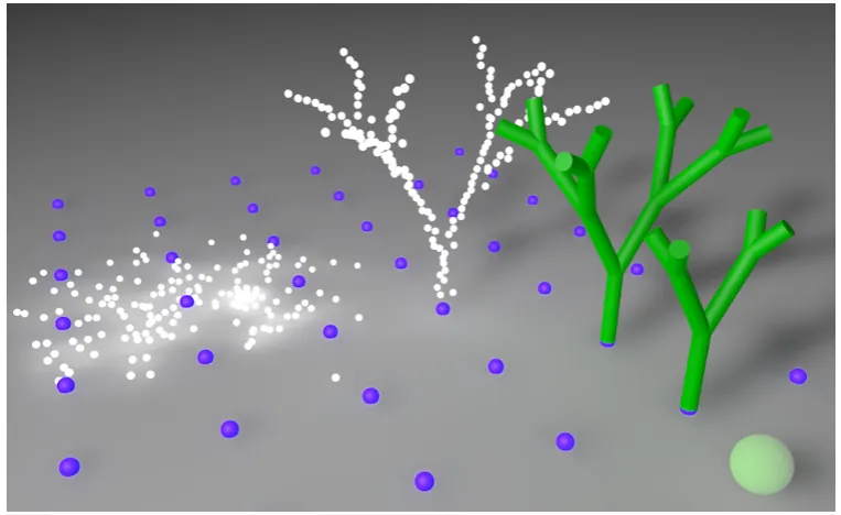
Figure2 shows the result of a more advanced example which combines XL with Dynamics and collision detection via CINEMA 4D’s built-in visual programming language XPresso: The large sphere rolls along the floor, and whenever it collides with one of the small grid points, this is detected by XPresso which then sets a user attribute on the grid point object. This in turn can be evaluated by XL to let a simple binary tree grow at such a point until it is eventually dissolved by XL into a set of light particles which fall down according to Dynamics.
5
Discussion
The structure of CINEMA 4D’s scene graph is well-suited for the application of XL. The shown examples could be adapted from their original GroIMP implementations [Kni09] without major changes, and they could easily be combined with advanced features like Dynamics. In fact, the GroIMP implementation of the polymerization has to include some simple simulation rules for monomer movement which are superfluous for XL4C4D. There are a lot more features from animation to sophisticated rendering from which one can benefit.
On the other hand, the Java Native Interface introduces a performance bottleneck, and CIN-EMA 4D isn’t able to handle very large amounts of objects or deep structures efficiently. So the system is not suitable for graphs of million nodes, which may appear in detailed plant models and which can be handled by GroIMP. E.g., for the classical example of the Koch snowflake curve, the plug-in allows only up to three iterations, reaching a graph depth of 384. Within GroIMP, nine iterations resulting in a depth of more than 1.5 million are possible without any problems.
Figure 2: The sphere triggers tree growth, eventually trees dissolve into light particles.
be realistic. Also the graph structures are typically relatively simple, but still too extensive to be modeled by hand. The last example can be seen as a (somewhat unskilled) representative of this kind of computer graphics.
XL4C4D operates on the scene graph level. A much more complex kind of 3D modeling happens at the deeper level of actual geometry. This is usually represented as a polygon mesh, i.e., another kind of graph. Typical operations on a mesh like extrusion [BPA+10] or subdivision [SMG10, BPA+10] can be modelled as graph transformations. We haven’t implemented such facilities for the plug-in, but it could be done based on the vv approach [SPS03,Kni09].
Bibliography
[BPA+10] T. Bellet, M. Poudret, A. Arnould, L. Fuchs, P. L. Gall. Designing a Topologi-cal Modeler Kernel: A Rule-Based Approach. In Shape Modeling International. Pp. 100–112. IEEE Computer Society, 2010.
[CJ92] T. W. Chien, H. J¨urgensen. Parameterized L Systems for Modelling: Potential and Limitations. In Rozenberg and Salomaa (eds.),Lindenmayer Systems. Pp. 213–229. Springer, Berlin, 1992.
[EEPT06] H. Ehrig, K. Ehrig, U. Prange, G. Taentzer. Fundamentals of Algebraic Graph Transformation. Springer, Secaucus, NJ, USA, 2006.
Com-parison with Double Pushout Approach. In Rozenberg (ed.), Handbook of Graph
Grammars and Computing by Graph Transformations, Volume 1: Foundations.
Chapter 4, pp. 247–312. World Scientific, 1997.
[KBHK08] O. Kniemeyer, G. Barczik, R. Hemmerling, W. Kurth. Relational Growth Gram-mars – A Parallel Graph Transformation Approach with Applications in Biology and Architecture. In Sch¨urr et al. (eds.),AGTIVE 2007. Lecture Notes in Computer Science 5088, pp. 152–167. Springer, 2008.
[KHK] O. Kniemeyer, R. Hemmerling, W. Kurth. GroIMP. http://www.grogra.de.
[Kni09] O. Kniemeyer.Design and Implementation of a Graph Grammar Based Language for Functional-Structural Plant Modelling. PhD thesis, BTU Cottbus, 2009.
[Kur94] W. Kurth. Growth Grammar Interpreter GROGRA 2.4 – A software tool for the 3-dimensional interpretation of stochastic, sensitive growth grammars in the context of plant modelling. Introduction and Reference Manual. Berichte des Forschungszen-trums Wald¨okosysteme, B 38, G¨ottingen, 1994.
[LR76] A. Lindenmayer, G. Rozenberg (eds.).Automata, Languages, Development. North Holland, Amsterdam, 1976.
[MAX] MAXON Computer GmbH. CINEMA 4D. http://www.maxon.net.
[Nag76] M. Nagl. On a Generalization of Lindenmayer-Systems to Labelled Graphs. Pp. 487–508 in [LR76].
[Nag79] M. Nagl. Graph-Grammatiken: Theorie, Anwendungen, Implementierungen. Vieweg, Braunschweig, 1979.
[PEM87] F. Parisi-Presicce, H. Ehrig, U. Montanari. Graph Rewriting with Unification and Composition. In Ehrig et al. (eds.), Third International Workshop on Graph-Grammars and Their Application to Computer Science. Lecture Notes in Computer Science 291, pp. 496–514. Springer, 1987.
[PKL07] P. Prusinkiewicz, R. Karwowski, B. Lane. The L+C plant modelling language. In Vos et al. (eds.), Functional-Structural Plant Modelling in Crop Production. Wa-geningen UR Frontis Series 22, pp. 27–42. Springer, 2007.
[PL90] P. Prusinkiewicz, A. Lindenmayer.The Algorithmic Beauty of Plants. Springer, New York, 1990.
[SMG10] A. Spicher, O. Michel, J.-L. Giavitto. Declarative Mesh Subdivision Using Topo-logical Rewriting in MGS. In Ehrig et al. (eds.),ICGT. Lecture Notes in Computer Science 6372, pp. 298–313. Springer, 2010.