Discovering Higher Level Structure in Visual SLAM
Andrew P. Gee, Denis Chekhlov, Andrew Calway and Walterio Mayol-Cuevas
Member, IEEE
Abstract—We describe a novel method for discovering and
incorporating higher level map structure in a real-time visual SLAM system. Previous approaches use sparse maps, populated by isolated features such as 3-D points or edgelets. Although this facilitates efficient localisation, it yields very limited scene representation and ignores the inherent redundancy amongst features resulting from physical structure in the scene. In this work, higher level structure, in the form of lines and surfaces, is discovered concurrently with SLAM operation and then incorporated into the map in a rigorous manner, attempting to maintain important cross covariance information and allow consistent update of the feature parameters. This is achieved by using a bottom-up process, in which subsets of low level features are ‘folded in’ to a parameterisation of an associated higher level feature, thus collapsing the state space as well as building structure into the map. We demonstrate and analyse the effects of the approach for the cases of line and plane discovery, both in simulation and within a real-time system operating with a hand-held camera in an office environment.
Index Terms—Higher level structure, kalman filtering, machine
vision, simultaneous localisation and mapping.
I. INTRODUCTION
V
ISUAL simultaneous localisation and mapping (SLAM) aims to use cameras to recover a representation of the environment that concurrently enables accurate pose estima-tion. Cameras are powerful additions to the range of sensors available for robotics, not only because of their small size and cost, but also for their ability to provide a rich set of world fea-tures, such as colour, texture, motion and structure. In mobile robotics, vision has proved to be an effective companion for more traditional sensing devices. For example, in [1], where vision is coupled with laser ranging, the visual information is reliable enough to perform loop-closure for an outdoor robot in a large section of an urban environment. Indeed, such is the utility of vision, that cameras have also been used as the main or only SLAM sensor, as demonstrated in the seminal work of Davison [2]–[4]. This enables applications for a wide range of moving platforms where the main mapping sensor could be a single camera, such as small domestic robots and a variety of personal devices. For these, visual SLAM offers the fundamental competence of beingspatially aware, a necessity for informed motion and task planning.A. Motivation
Although there have been significant advances in visual SLAM, these have been primarily concerned with locali-sation. In contrast, progress in developing mapping output
Manuscript received December 18, 2007; revised July 18, 2008. The work of A. P. Gee was supported by the EPSRC Equator IRC. The work of D. Chekhlov was supported by ORSAS, University of Bristol Postgraduate Research Scholarship and the Leonard Wakeham Endowment.
The authors are with the Department of Com-puter Science, University of Bristol, UK (email:
{gee,chekhlov,andrew,wmayol}@cs.bris.ac.uk)
has been somewhat neglected. Systems have been based on maps consisting of sparse, isolated features, predominantly 3-D points [2], [5], [6], but also 3-3-D edges [7]–[9] and localised planar facets [10]. Such minimal representations are attractive from the localisation point of view. With judicious choice of features, image processing can be kept to a minimum, enabling real-time operation whilst maintaining good tracking performance. Recent work has further improved on localisa-tion to give better robustness by adopting different frameworks such as factored sampling [11], by using more discriminative features [6], [12], or by incorporating re-localisation methods for when normal tracking fails [5]. Whilst this has certainly improved performance significantly, the information contained in the resulting maps is still very limited in terms of the representation of the surrounding environment. In this paper we seek to address this issue by investigating mechanisms to discover and then incorporate higher level map structure, such as lines and surfaces, in visual SLAM systems.
B. Related Work
The detection of higher level structure has been considered before, using both visual and non-visual sensors. In most cases this happens after the map has been generated. For example, in [13], [14], planes are fitted to clouds of mapped points determined from laser ranging. However, the discovered structures are not incorporated into the map as new features and so do not benefit from correlation with the rest of the map and must be re-fitted every time that the underlying map changes.
In other examples, higher level features are recoveredbefore
they are added into the map, such as those described in [15]– [17], where 2-D geometric primitives are fitted to sonar returns and then used as features, and [18], [19] where 3-D planes are fitted to laser range data. The method described in [20], [21] takes this approach a stage further and fuses measurements from a laser range finder with vertical lines from a camera to discover 2-D lines, semi-planes and corners which can be treated together as single features. In [22] visual map features, such as lines, walls and points, are represented in a Measurement Subspace which can vary its dimensions as more information is gathered about the feature.
In vision based SLAM, maps have been enhanced by virtue of users providing annotations [23], [24], manually initialising regions with geometric primitives [25] or by embedding and recognising known objects [26]. These systems require user intervention and importantly, the structures are not able to grow to include other features as the map continues to expand.
C. Contribution
In contrast to the above, we propose a system in which higher level structure is automatically introducedconcurrently
with SLAM operation, and importantly, the newly discovered structures become part of the map, co-existing seamlessly with existing features. Moreover, this is done within a single framework, maintaining full cross covariance between the different feature types, thus enabling consistent update of feature parameters. This is achieved by augmenting the system state with parameters representing higher level structures, in a manner similar to that described in [20], [21]. The novelty of the approach is that we use existing features in the map to infer the existence of higher level structure and then proceed to ‘fold in’ subsets of lower order features which already exist in the system state and are consistent with the parameterisa-tion. This collapses the state space, reducing redundancy and computational demands, as well as giving a higher level scene description. The approach therefore differs both in the timing at which higher level structure is introduced and in the way the newly discovered structure is maintained and continually extended.
The paper is organised as follows. We first introduce a generic SLAM framework, based around Kalman filtering, in which higher level structure can be incorporated into a map concurrently with localisation and mapping. This is followed by details of how this can be achieved for the cases of planes and lines, based on collapsing subsets of 3-D points and edgelets, respectively. Results of experiments in simulation and for real-time operation using a hand-held camera within an office environment are then presented, including an analysis of the different trade-offs within the formulation. The paper concludes with a discussion on the directions for future work. Initial findings of the work were previously reported in [27].
II. VISUALSLAMWITHHIGHERLEVELSTRUCTURE
We assume a calibrated camera moving with agile mo-tion whilst viewing a static scene. The aim is to estimate the camera pose, whilst simultaneously estimating the 3-D parameters of structural features, such as points, lines or surfaces. This is done using a Kalman filter framework. The system state x = [v,m]T has two partitions, one for the
camera pose v = [q,t]T and one for the structural features,
m = [m1,m2, . . .]T. The camera rotation is represented by
the quaternionqandtis its 3-D position vector, both defined w.r.t a world coordinate system. We adopt a generalised framework for the structural partition to allow multiple feature types to be mapped. Each mi denotes a parameterisation of
a feature, for example a position vector for a 3-D point or the position and orientation of a planar surface. In general, we expect the number and the types of features to vary as the camera explores the environment, with new features being added and old ones being removed so as to minimise computation and maintain stability.
A. Kalman Filter Formulation
The Kalman filter requires a process model and an obser-vation model, encoding the assumed evolution of the state between time steps and the relationship between the state and the filter measurements, respectively [28]. Application of the filter to real-time visual SLAM is well documented (see e.g.
[2], [6], [29]); we therefore provide only a brief outline here. We assume a constant position model for the camera motion, i.e. a random walk, and since we are dealing with a static scene this gives the process model
xnew=f(x,w) = [∆q(wω)⊗q,t+wτ,m]T (1)
wherew = [wω,wτ]T is a 6-D noise vector, assumed to be
from N(0,Q),∆q(wω) is the incremental quaternion
corre-sponding to the Euler angles defined by wω, and ⊗ denotes
quaternion multiplication. Note that the map parameters are predicted to remain unchanged (we assume a static scene) and that the non-additive noise component in the quaternion part is necessary to give an unbiased distribution in rotation space. At each time step, we collect a set of measurements from the next frame obtained from the camera, z= [z1,z2, . . .]T,
where in general each zi will be related to the state via a
separate measurement function, i.e.zi =hi(x,e), where eis
a multivariate noise vector fromN(0,R). For example, when mapping point features, the measurements are assumed to be corrupted 2-D positions of projected points and for the ith measurement
hi(x,e) = Π(y(v,mj)) +ei (2)
wheremj is the 3-D position vector of the point associated
with the measurement zi, y(v,mj) denotes this position
vector in the camera coordinate system, Π denotes pin-hole projection for a calibrated camera andeiis a 2-D noise vector
fromN(0,Ri).
Application of the filter at each time step gives mean and covariance estimates for the state based on the process and observation models. Both of these are non-linear and thus we use the extended Kalman filter (EKF) formulation, in which updates are derived from linear approximations based on the Jacobians off andhi[28]. The role of the covariances
within the filter is critical. Proper maintenance ensures that updates are propagated amongst the state elements, particularly the structural components, which are correlated through their mutual dependence on the camera pose [30], [31]. This ensures consistency and stability of the filter. Propagation of the state covariance through the observation model also allows for better data association, constraining the search for image features. As discussed next, it is therefore crucial to ensure that covariances are properly maintained for successful filter operation.
B. Augmenting and Collapsing the State
We adopt a bottom up process in order to incorporate higher level structure into a map. This works as follows. Given a map populated by isolated lower level features, we seek subsets which support the existence of higher level structure such as lines or surfaces. With sufficient support, a parameterisation of the higher level feature is then augmented to the state, with an initial estimate derived from the supporting features. Subsequently, lower level features consistent with the parameterisation are linked to that feature and transformed according to the constraint that it imposes. This results in a
collapsing of the state space, reducing redundancy. Details of how this is achieved in practice are given in Section III.
A key aspect of the work described in this paper is that the above process is implemented in a rigorous manner within the filter. For this we draw on the procedures for transforming and expanding states [32], which also forms the basis for initialising isolated features in existing systems [33]. Aug-mentation and collapsing of the state is done in such a way so as to preserve full correlation amongst existing and new features within the map. This ensures that parameter updates are carried out in a consistent fashion. It can be formalised as follows. Assume that we have an existing state estimate
ˆ
x= [ˆv,mˆ1, . . . ,mˆn]T, where there arenfeatures in the map,
and that we wish to augment the state with a new (higher level) feature mn+1, based on an initialisation measurement zo. In
general, the initial estimate for the feature will be derived from a combination of the measurement and the existing state, i.e.
ˆ
mn+1 = s(ˆx,zo), and the augmented state covariance then
becomes Pnew = J P 0 0 Ro JT (3) J= " I 0 ∇sv ∇sm1 . . . ∇smn ∇szo # (4) where Ro is the covariance of the measurement and ∇sv = ∂s/∂v. Thus, the covariance matrix grows as illustrated in Fig. 1 and introduces the important correlations between the new feature and the existing features in the map. For example, in the case of augmentation with a new planar feature derived from a subset of point features, only the relevant Jacobians
∇smi will be non-zero and the feature will be correlated with
the camera pose through that subset of points.
In a similar way, we can also transform an existing feature to a different representation, e.g.mˆnew
i =r(ˆx), and then the
covariance update is given by
Pnew=JPJT (5) J= I 0 0 ∇rv . . . ∇rmi . . . ∇rmn 0 0 I (6)
where any change in the dimensions of the state is reflected in the dimensions of the Jacobian J.
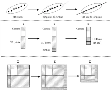
Both of the above relationships allow us to introduce higher level features and collapse the state size whilst maintaining the cross correlations within the filter. For example, as illustrated in Fig. 1, consider a new feature mn+1 which represents
a higher level structure and which imposes a constraint on a subset of existing features (a line and a set of points, respectively, in Fig. 1). Given an initial estimate ofmn+1, we
can introduce it into the system using (3) and the constraint can then be imposed by transforming the existing features into the new constrained representation using (5). This collapses the state by removing redundant constrained variables, whilst also maintaining the correlations between the new features, the camera pose and the remainder of the map.
000 000 000 000 000 111 111 111 111 111 00 00 00 00 00 00 00 00 11 11 11 11 11 11 11 11 0000000 0000000 0000000 0000000 0000000 1111111 1111111 1111111 1111111 1111111 0000000 0000000 0000000 0000000 0000000 1111111 1111111 1111111 1111111 1111111 000000000000000 11111 11111 11111 000000000 000000000 000000000 111111111 111111111 111111111 000 000 000 000 000 000 000 000 000 000 000 111 111 111 111 111 111 111 111 111 111 111 000000000 000000000 000000000 111111111 111111111 111111111 000 000 000 000 000 000 000 000 000 000 000 111 111 111 111 111 111 111 111 111 111 111 00 00 00 11 11 11 00 00 00 00 00 00 00 11 11 11 11 11 11 11 000 000 000 111 111 111 000 000 000 000 000 000 000 111 111 111 111 111 111 111 00 00 00 11 11 11 00 00 00 11 11 11 00000 00000 00000 11111 11111 11111 0000000 0000000 0000000 0000000 1111111 1111111 1111111 11111110000 00 00 00 00 00 00 00 00 00 00 00 00 11 11 11 11 11 11 11 11 11 11 11 11 11 11 000000000 000000000 000000000 000000000 000000000 000000000 000000000 111111111 111111111 111111111 111111111 111111111 111111111 111111111 000000 000000 000000 111111 111111 111111 000 000 000 000 000 000 000 111 111 111 111 111 111 111 000000000 000000000 000000000 000000000 000000000 000000000 000000000 111111111 111111111 111111111 111111111 111111111 111111111 111111111 000000 000000 000000 111111 111111 111111 000 000 000 000 000 000 000 111 111 111 111 111 111 111 000000000000 000000000000 000000000000 000000000000 111111111111 111111111111 111111111111 111111111111 00 00 00 00 00 00 00 00 00 00 00 00 00 00 00 00 00 00 00 00 00 00 00 00 11 11 11 11 11 11 11 11 11 11 11 11 11 11 11 11 11 11 11 11 11 11 11 11 000 000 000 111 111 111 00 00 00 11 11 11 00 00 00 11 11 11 00 00 00 00 11 11 11 11 x Camera x
3D points 3D points & 3D line
Camera x 3D line 3D points 3D line 3D points Camera Σ Σ Σ
3D line & 1D points
1D Points 00 00 00 00 11 11 11 11 00 00 00 00 11 11 11 11
Fig. 1. Collapsing the state space when introducing higher level structure into the SLAM map: (left) map consists of point features; (middle) parame-terisation of higher level line feature introduced into the map, expanding the statexand the covarianceΣ; (right) state space collapses as points on the line are ‘folded in’ to the higher level feature.
III. BUILDING INHIGHERLEVELSTRUCTURE
In practice, building higher level structure into a system map has three distinct components: discovery - determining subsets of isolated features that support the premise that a higher level structure is present;incorporation- initialising a parameterisation of the higher level feature into the system state and linking existing features to it; and measurement -deriving measurements for the higher level feature in order that it and its linked features can be updated within the filter.
A. Discovery
The discovery component is essentially a segmentation task amongst existing features in a map and we adopt a RANSAC approach [34]. This involves generating hypotheses from minimal sets of features randomly sampled from the subset of features having sufficient convergence, i.e. with variance less than some suitable threshold, σRAN SAC2 . Each hypothesis is then tested for consensus with the rest of the set. Thus, given a minimal set of features,(m1,m2, . . . ,mK),
we generate the parameters for a higher level feature viap=
g(m1,m2, . . . ,mK)and a featuremiis then deemed to be in
consensus with the hypothesis if a distance measured(p,mi)
from the hypothesised feature is less than some threshold,
dRAN SAC. The choice of thresholds here is important and essentially controls the system’s willingness to introduce new structure into the map. We discuss this further and analyse the trade-offs in Section V.
In practice, RANSAC search is not performed over the global map but using a small local set of the N most recently observed features. At the beginning of each search, a random feature from this set is chosen as a base reference and used to temporarily transform the other features in the set and discover their relative uncertainties, using the technique described in [17]. The local covariances of the features are used for thresholding, allowing the discovery of local structure even
when the global uncertainty is large. We use a standard imple-mentation of RANSAC and do not currently use the variance information within the algorithm itself, although this could be incorporated in the future, e.g. by temporarily transforming features prior to a Mahalanobis distance consensus test by using the hypothesised higher-level features as a base frame of reference.
B. Incorporation
The hypothesis with the most consensus yields a set of in-lying features from which ‘best-fit’ parameters can be derived in order to initialise the associated higher level feature. This marks the start of the incorporation component.
First, a χ2 similarity test with 95% bounds is performed to ensure that the proposed higher level structure is not too similar to any existing structures in the system. If the test is passed then the state is augmented with the initial parameter estimates and the covariance is then expanded according to (3), wheres(x,zo)denotes the derivation of the parameters from
the set of inlying features. Note that since the parameters are derived only from the inliers, then bothzo=0and∇sv=0,
and we need only compute the Jacobians∇smi. This ensures
that the parameters are correlated with the rest of the SLAM state through the inlying features.
Having initialised a higher level feature, the system then seeks to link existing features to it and transform them according to the constraint that it imposes. Whilst we could immediately incorporate all of the inlying features into the new structure, we choose not to do this because the current RANSAC search does not fully take into account the uncer-tainty of the features, as discussed in Section III-A. Instead, we gradually add features to the structure, adopting the following procedure for each feature in the map (or a local subset of features around the new structure):
1) Temporarily transform the feature using the new struc-ture as a base reference [17] to give us the state and covariance relative to the new structure.
2) Reject the feature if σ2
max > σ2T, where σmax is the
maximum std. deviation of the feature relative to the structure, andσT is a threshold std. deviation.
3) Reject the feature if d(p,mi) > dT, where d(p,mi)
is a measure of the distance from the structure, e.g. the RANSAC consensus distance measure, and dT is a distance threshold.
4) Acceptthe feature if its Mahalanobis distance from the structure is less than the 95%χ2 threshold.
Features accepted for incorporation are transformed into a new representation, e.g. mˆnewi = r(ˆx), and the state covariance updated according to (5). This typically results in a collapsing of the state due to the constraint imposed by the higher level feature. For example, as described in the next section, 3-D point features linked to a planar feature are transformed into 2-D points lying on the plane.
It is important to emphasise that once the higher level feature is added to the map, we are able to continue to seek for new features to link to it, even if they were not initially used to estimate the higher level feature or were subsequently added to the map after incorporation.
C. Measurement
The parameters for both the higher level feature and its linked features are updated in the usual manner within the filter. To do so, we require an observation function, linking the parameters to measurements obtained from the incoming image frames. The details of this function will be dependent on the type of higher level features and specific examples are given in Sections IV-A4 and IV-B4 for the cases of planes and lines respectively. Due to the cross-covariance terms introduced between features and the higher-level struc-ture, measurement of one will necessarily update the other. Therefore, it is possible to update the higher level feature even if we are unable to take direct measurements of it.
IV. PLANES ANDLINES
In this section, we describe the specific cases of discovering and incorporating planar and straight line structure within maps consisting of isolated 3-D points and edgelets, respec-tively. The mechanisms closely follow the steps described in Section III. We therefore only note the key differences and implementation details here.
A. 3-D Planes from Points
In the case of planes, we aim to discover the location, extent and orientation of planar structure formed by 3-D points being concurrently mapped. Once a plane has been initialised, 3-D points deemed to be consistent with it are collapsed into 2-D planar points, reducing the state size, and may even have their location on the plane fixed so that the point can be completely removed from the state. Note, however, that since we are interested in reducing redundancy in the system, we do not at present verify that the discovered planes correspond to physical planes in the scene (c.f. Section VII).
1) Representation : Since we want to use the plane as a coordinate frame for 2-D points which are ‘folded into’ the plane, we need to parameterise the orientation of the plane around its normal direction as well as its origin. For convenience we use a non-minimal representation with a 9-D state vector, so that a new planar feature augmented to the state has the form mn+1 = [po,c1,c2]T, where po is the
plane origin and the orientation is defined by two orthonormal basis vectors,c1 andc2, which lie on the plane. The normal
to the plane is then simply the cross product between the two basis vectors, i.e.n=c1×c2. A 3-D point in the map which
is deemed to lie on the plane and whose feature vector mi
defines its 3-D position vector, can then be transformed into a 2-D planar point using
mnewi = [(mi−po) · c1, (mi−po) · c2]T (7)
where · denotes the dot product. Thus for l such points on a plane, this gives a state size of 9 + 2l, compared with 3l, giving a reduction in state size for l > 9. In the filter, the orthonormality constraint of the basis vectors is applied after every update, by displacing the mean to satisfy the constraint and updating the covariance to reflect this displacement (c.f. the ‘displOff’ algorithm in [35]).
2) Discovery: The discovery of potential planar structure using the RANSAC process is similar in approach to that used in [36]. We require a minimum of three 3-D points to generate the parameters for a plane hypothesis, i.e.
po=m1 c1=m2−m1 c2=m3−m1 (8)
Consensus for the hypothesis amongst other points is then determined using a distance measure based on perpendicular distance from the plane, i.e. for a point mi, the distanced=
(mi−po)·n.
We also impose the additional criterion that the Euclidean distance from the plane origin must be less than a second threshold dmax, which ensures that we only initialise planes with strong local support. This biases the system towards introducing planes which are likely to match local physical structure, rather than fitting a geometric plane through a dis-perse set of points. This is beneficial because it is reasonable to assume that a physical plane will contain other, currently undiscovered, co-planar points which can be ‘folded in’ to the plane in the future.
To determine the best fit plane from the inliers resulting from the RANSAC process, we use a principal component approach similar to [19]. The origin is set to the mean and the orientation parameters are determined from the principal components. Specifically, if the position vectors for l inlying points w.r.t the mean are stacked into an l ×3 matrix M, then the eigenvector of MTM corresponding to the smallest eigenvalue gives the normal to the plane and the other two eigenvectors give the basis vectors within the plane. The smallest eigenvalue, λmin, is the variance of the inliers in the normal direction and provides a convenient measure of the quality of the fit. It is possible for this approach to return poorly conditioned eigenvectors if the system is degenerate. This case can be tested for by rejecting planes with pairs of similar eigenvalues.
3) Incorporation: In order to avoid adding poor estimates of planes to the system state, the best-fit plane generated by the RANSAC process is only initialised ifl > lT andλmin< λT. The best-fit parameters are used to initialise a plane feature in the state and the covariance is updated according to (3), where the Jacobian w.r.t an inlying point featuremi is computed as:
∇smi= ∂p o ∂mi , ∂c1 ∂mi , ∂c2 ∂mi T (9) where ∂c1/∂mi and ∂c2/∂mj are the Jacobians of the two
eigenvectors computed using the method described in [37]. This ensures that the plane parameters are correlated with the rest of the state through the inlying point features.
As an additional criterion for incorporation of the point onto the plane, we reject the point if its distance from the plane origin or any other point on the plane is greater than
dmax. Again, this is to bias the system towards accepting local
planes.
4) Measurement : We do not consider here making a direct observation of the plane. Instead, we base the plane measurement on observations of the 2-D points linked to the plane. The measurement model for a 2-D planar point mi
is very similar to that of a standard 3-D point feature, but
involves an additional preliminary step to convert it to a 3-D position vector pin the world frame of reference prior to projection into the camera, i.e. from (7)
p= [c1 c2]mi + po (10)
The predicted measurement for the planar point can then be obtained by passing p through the standard perspective pro-jection model in (2). The similarity between the measurement models makes the implementation of planar points in the considered EKF SLAM system very simple. The measurement Jacobian required by the EKF is much the same as that for 3-D point features, except that we need to take account of the conversion in (10) when computing the Jacobian relating the observation to the 2-D point feature, i.e
∂hi ∂mi = ∂hi ∂p ∂p ∂mi (11) where hi is the measurement function associated with a
3-D point (2) and ∂p/∂mi is the Jacobian of the 3-D point
w.r.t the 2-D planar point, derived from (10). Finally, since the predicted observation is also dependent on the position and orientation of the plane, a Jacobian∂hi/∂mj relatinghi
to the relevant plane featuremj is also derived from (10).
5) Fixing Plane Points : If the maximum of the variances of a 2-D planar point becomes very small relative to the plane, i.e. less than a threshold σf ix, then we can consider further collapsing the state space by removing it completely from the state. Instead of maintaining an estimate of its 2-D position on the plane, we consider it as a fixed point in the plane and use its measurements to update the associated planar feature directly. This leads to further reduction in the size of the state space.
B. 3-D Lines from Edgelets
Another natural option to enhance scene description beyond sparse points are edges. In this case we consider edgelet features, which are locally straight sections of a gradient image proposed in [7]. An edgelet is composed of a point in 3-D and its direction. By their nature, edgelets can be initialised along a variety of edge shapes by assuming that even curved edges can be approximated by locally straight sections. In this case, we are interested in discovering straight lines formed from collections of edgelets and perform a reduction in state size similar to that of points incorporated into planes.
1) Representation: We parameterise an edgelet in 6-D, composed of its 3-D position, ce, and unnormalised 3-D
direction vector, de. Similarly, a 3-D line feature is defined
by mn+1 = [cl,dl]T, where cl denotes its origin point and
dlis its direction.
2) Discovery: In the RANSAC discovery component, we use a minimal set of two edgelets to generate line hypotheses, based on their 3-D position vectors, which we found to give more reliable results than using a single edgelet. The consensus distance measure is then based on the perpendicular distance of an edgelet’s 3-D position from the line and the difference in its 3-D orientation. Principal components of the inlier set with most consensus then provides an initial estimate of the line direction and the mean 3-D position of the inliers is taken as the line origin.
3) Incorporation: After a line is put in the state, edgelets deemed to lie on the line are linked to it and transformed into 1-D line points parameterised by their distance from the line origin. These 1-D edgelets can then be removed from the state, reducing the state size dramatically. Transforming directly from the 6-D edgelet representation to a fixed, 1-D representation on the line makes sense because the remaining degree of freedom, which allows the edgelet to move along the line, is not observable in the edgelet measurements [7], which only measure perpendicular offset from the line. Also, the edgelet does not have a descriptor linking it to a specific point on the line, so small errors in position along the line will have no effect on the performance of the system. This is a marked contrast to the case of points on a plane, where each point measurement is associated through a visual descriptor to specific feature in the image. To transform the edgelet, we simply project it onto the line along the perpendicular direction.
4) Measurement : In contrast to the case with planes, we do not pass all of the individual observations of the line points into the EKF. Instead, a single observation for the line is computed by projecting each of its fixed edgelets into the image plane (with 3-D orientation set to that of the line) and applying a RANSAC line-fitting method to robustly fit a single line to individual edgelet measurements. The direction and position of this single line in the image is passed into the EKF as the observation of the 3-D line. Measurement Jacobians for the EKF are then computed in a similar manner to (11).
This approach has two distinct benefits: i) the number of observations which the EKF has to process each frame is significantly reduced; andii)the RANSAC line-fitting ensures that we only accept mutually compatible measurements of the edgelets along the line, similar to the mutual compatibility test between the features of a given landmark in [21].
V. SIMULATIONS
A. Methodology
We have analysed the approach using two different simu-lated environments. The simulations model a 6 d.o.f. camera moving through space with a 81◦ horizontal f.o.v. and image size 320 ×240 pixels. The simulated data has been used to measure the system consistency and the accuracy of the tracking and reconstruction against the known ground truth. In each case, the simulated environment contains a small set of known landmarks which are initially visible from the camera. This ‘template’ provides a known scale for the map.
1) Consistency: The consistency of the system is measured using the normalised estimation error squared (NEES) [28] averaged over multiple Monte Carlo runs of the simulations. If the system is consistent, then we expect this average value to converge towards the dimension of the system state, which we can test using aχ2test with 95% bounds. An average value above the upper bound indicates that the system is optimistic, a case which we particularly want to avoid because it reduces the positive effects of loop-closure and prevents successful data association if we use feature innovation to constrain the search for image features.
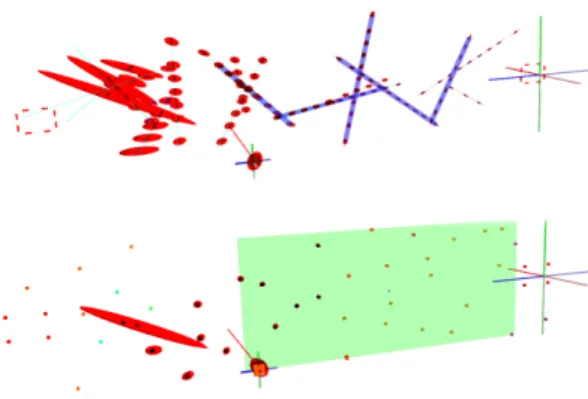
Fig. 2. Small map simulation results: (top) edgelet mapping and line discovery; (bottom) point mapping and plane discovery. A known template of points/edgelets is positioned at the beginning and end of the wall to give a known scale to the map and provide loop closure at each end. Covariance is drawn as red ellipsoids. Ground-truth lines are drawn in pale red/cyan according to whether they are currently observed by the camera, and the estimated lines are superimposed on top as thicker blue lines. The estimated plane is drawn using a pale green bounding box around the included points. Full sequence videos and a PDF version of this article with colour images are available in IEEE Xplore.
TABLE I
PLANE AND LINE SIMULATION RESULTS OVER50RUNS ON A SMALL MAP
Scenario Inconsistent Pos MAE Ang MAE State Red.
% frames cm radians % max
No Lines 0.0 0.07±0.06 0.06±0.05 0.0±0.0 Lines 0.0 0.05±0.06 0.01±0.01 97.9±0.1 No Planes 0.0 0.05±0.04 - 0.0±0.0 Planes A 0.0 0.04±0.03 - 21.5±0.4 Planes B 0.2 0.41±0.37 - 21.3±3.1 Planes C 0.1 0.41±0.39 - 47.7±9.8
Table 1. Plane and line simulation results over 50 runs on a small map with two loop closures, showing camera consistency, final mean absolute map error (MAE) in position and angle, and percentage state reduction. Planes A - no clutter; Planes B - with clutter; Plane C - as B, but with plane points converted to fixed points.
2) State Size Reduction: The state size reduction from adding higher level features is expressed as a percentage of the maximum reduction we could achieve if all of the simulated features initialised on ground-truth higher level structures were added correctly to their higher level structure by the system. For example, in a simulation of a set of points initialised to lie on a plane, we would achieve 100% of the maximum state size reduction if all of these points were successfully added to one discovered plane in the system map.
B. Small Map Simulation
The first simulation (Table I, Fig. 3 and Fig. 4) demonstrates the improvement in mean absolute error of the map and reduction in state size caused by adding higher level structure in a small map with multiple loop closures, as might be typical in a desktop visual SLAM system or within a local map of a submapping SLAM system. The environment contains ground-truth line or point features arranged randomly in a 4m long volume and the camera translates along a sinusoidal path in front of them (Fig. 2). The positions of newly observed points and edgelets are initialised as 6-D inverse depth points [33] and converted to 3-D points once their depth uncertainty
0 1 2 3 4 5 6 7 8 0 500 1000 1500 2000 NEES frame Lines - Small Map Simulation - Camera NEES (50 runs)
No Lines Lines 0 0.5 1 1.5 2 2.5 3 0 200 400 600 800 1000 1200 1400 1600 1800 2000 cm 2 frame
Lines - Small Map Simulation - Camera Position MSE (50 runs)
No Lines Lines 0 0.01 0.02 0.03 0.04 0.05 0 500 1000 1500 2000 cm 2 frame
Lines - Small Map Simulation - Feature Map Position MSE (50 runs)
No Lines Lines 0 0.002 0.004 0.006 0.008 0.01 0.012 0.014 0 500 1000 1500 2000 radians 2 frame
Lines - Small Map Simulation - Feature Map Orientation MSE (50 runs)
No Lines Lines
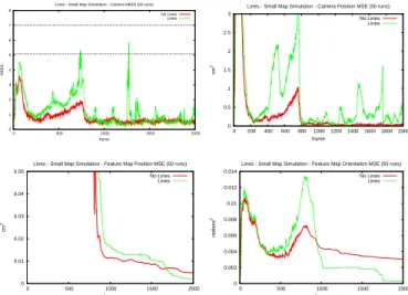
Fig. 3. Small map simulation results for lines over 50 Monte Carlo runs: (top-left) average camera NEES remains below upper threshold indicating that the camera does not become inconsistent; (top-right, left, bottom-right) evolution of MSE for the camera position, edgelet positions and edgelet orientations respectively. Loop closure occurs around frame 750.
0 2 4 6 8 10 0 500 1000 1500 2000 NEES frame Planes - Small Map Simulation - Camera NEES (50 runs)
No Planes Planes A - no outliers added to plane Planes B - standard plane discovery Planes C - points fixed on plane
0 0.2 0.4 0.6 0.8 1 1.2 0 500 1000 1500 2000
num inconsistent features / num features
frame Planes - Small Map Simulation - Map Consistency (50 runs)
No Planes Planes A - no outliers added to plane Planes B - standard plane discovery Planes C - points fixed on plane
0 0.5 1 1.5 2 0 500 1000 1500 2000 cm 2 frame
Planes - Small Map Simulation - Camera Position MSE (50 runs) No Planes Planes A - no outliers added to plane Planes B - standard plane discovery Planes C - points fixed on plane
0 0.05 0.1 0.15 0.2 0.25 0.3 0 500 1000 1500 2000 cm 2 frame
Planes - Small Map Simulation - Feature Map Position MSE (50 runs) No Planes Planes A - no outliers added to plane Planes B - standard plane discovery Planes C - points fixed on plane
Fig. 4. Small map simulation results for planes over 50 Monte Carlo runs: (top-left) average camera NEES remains below upper threshold indicating that the camera does not become inconsistent; (top-right) proportion of features which are inconsistent increases after loop closure if outliers are erroneously added to the plane; (bottom-left, bottom-right) evolution of MSE for the camera position and map respectively. Loop closure occurs around frame 750.
becomes Gaussian [38]. We assume perfect data association and Gaussian measurement noise of 0.5pixel2. Thresholds for the planes were set at: dT = 0.1cm; σT = 1.0cm; σRAN SAC = 2σT; dmax = 200cm; and lT = 7. Thresholds
for lines were set at: dT = 0.5cm,24◦; σT = 1.0cm,24◦; σRAN SAC = σT; dmax = 120cm; and lT = 4. The
other thresholds were set in relation to these first ones as:
dRAN SAC =dT;λT =d2T; andσf ix=dT.
In the line simulations, the values in Table I correspond to a significant mean reduction in state size from 780 to 204. The mean absolute error in orientation and position is also improved by adding lines, as shown in Fig. 3. In particular, the relatively large covariance on edgelet direction measurements and limited motion of the camera means that the edgelets do
Fig. 5. Plane simulation results for Planes B: (far-left) initial point mapping and plane discovery; (centre-left) large covariance prior to loop closure; (centre-right) covariance and map error reduction after loop closure; (far-right) further reduction in covariance and slight inconsistency after second loop. Point and camera covariance shown in red and plane covariance in blue. Green lines denote ground-truth walls and estimated planes shown as blue bounding boxes around included points, with thickness indicating angle error. A full sequence video and a PDF version of this article with colour images is available in IEEE Xplore.
TABLE II
ROOM SIMULATION RESULTS OVER30RUNS ON A ROOM MAP
Scenario Inconsistent Pos MAE State Red.
% frames cm % max No Planes 4.8 3.0±2.2 0.0±0.0 Planes D 4.3 3.0±2.3 −27.1±3.6 Planes E 7.3 3.2±2.3 22.9±2.2 Planes B 21.6 3.6±2.7 22.2±2.5 Planes C 24.1 3.6±2.3 25.1±3.3
Table 2. Room simulation results over 30 runs on a larger map with two loop closures, showing camera consistency, final mean absolute map error (MAE) and state reduction. Planes B - with clutter; C - as B, but plane points converted to fixed points; Planes D - planes only, no incorporation of points; Plane E - as B, but discovery started after first loop closure.
not quickly converge to a good estimation on their own, so applying a line constraint helps to overcome these limitations. In the plane simulations we also investigated adding clutter around the plane, by positioning 50% of the points randomly within ±20cm of the ground-truth plane (Planes B in Table I). When clutter points are prevented from being added to the plane using ground-truth knowledge (Planes A), the results in Fig. 4 show similar characteristics to the line experiments, demonstrating reduction in mean absolute error and state size and no significant effect on consistency of the camera or the map. When clutter points are allowed to be erroneously added to the plane (Planes B and C), this performance degrades due to the added inconsistency in the map that becomes visible at loop closure (around frame 750, Fig. 4). However, the system still achieves0.4cm accuracy over a4m map and is capable of respectable state size reductions when points are fixed on the plane.
C. Room Simulation
In the second simulation the camera moves through a larger environment with 3-D points randomly arranged on and around the walls of a4msquare room (Fig. 5). Clutter distribution and thresholds are left the same as for the previous experiments (c.f. Section V-B). The challenge in this simulation is that loop closures occur less regularly and camera orientation error is given time to grow much larger.
When we allow the map to converge before adding higher level structure (Planes E), then consistency and mean absolute error is comparable to points only operation (No Planes), as
0 2 4 6 8 10 12 14 0 1000 2000 3000 4000 5000 NEES frame Planes - Room Simulation - Camera NEES (30 runs)
No Planes Planes D - planes added, points not added to planes Planes E - planes added after 1st loop Planes B - standard plane discovery Planes C - points fixed on plane
0 0.2 0.4 0.6 0.8 1 1.2 0 1000 2000 3000 4000 5000
num inconsistent features / num features
frame Planes - Room Simulation - Map Consistency (30 runs)
No Planes Planes D - planes added, points not added to planes Planes E - planes added after 1st loop Planes B - standard plane discovery Planes C - points fixed on plane
Fig. 6. Consistency results over 30 Monte Carlo runs for the room simulation: (left) average NEES of the camera state, the horizontal lines indicate the 95% bounds on the average consistency and the system is inconsistent if the NEES exceeds the upper bound; (right) proportion of points in the map with optimistic average consistency at each frame. Loop closure occurs around frames 2700 and 5400.
shown in Table II, Fig. 6. However, we get the additional benefit of reduced state size and improved understanding of the environment. Similar performance is achieved when we add planes to the map but don’t incorporate points onto the plane (Planes D): consistency and mean absolute error are preserved, although in this case the state size increases since planes are added but no points are removed.
Differences in consistency only occur when the system attempts to incorporate points before loop closure (Planes B, C in Fig. 6). In these cases, mean absolute error is slightly larger but still comparable to the other cases. It seems as though the additional inconsistency is caused by a combination of two factors: adding outlier points to the plane; and introducing errors when projecting 3-D points onto the plane to enforce the planarity constraint. We intend to investigate this further in future work.
VI. REALWORLDEXPERIMENTS
A. Methodology
To illustrate the operation of the approach with real world data we present results obtained for plane discovery from points within a real-time visual SLAM system. This operates with a hand-held camera and experiments were carried out in an office environment containing textured planar surfaces. We use a firewire web-cam with frames of size 320×240
pixels and a 43◦ FOV. The system begins by mapping 3-D points, starting from known points on a calibration pattern [2]. As the camera moves away, new points are initialised and added to the map, allowing tracking to continue as the camera explores the scene. Points are added using the inverse depth representation [33] and augmented to the state in a manner which maintains full covariance with the rest of the map [39] (c.f. section II-B). For measurements, we use the FAST salient point detector [40] to identify potential features and SIFT-like descriptors with scale prediction [12] for repeatable matching across frames.
B. Results
Fig. 7 shows results from an example run. On the left are external views of the estimated camera position and map estimates in terms of 3-D points and planes at different time frames. The images on the right show the view through the camera with mapped point and planar features superimposed.
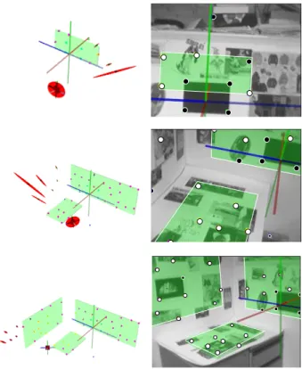
Fig. 7. Examples from a run of real-time visual SLAM with plane discovery using a hand-held camera in an office environment: (left) view of estimated camera position, 3-D mapped points and planar features; (right) views through the camera with discovered planar features superimposed (boundaries in white) with converged 3-D points in black and 2-D planar points in white. A full sequence video is available in IEEE Xplore.
Fig. 8. Convergence of planar features within the SLAM framework. Note the reduction in the graphic thickness for the left wall plane, indicating a reduction in uncertainty of plane position and orientation.
Note that the three planes in the scene have been successfully discovered and incorporated into the map. The vast majority of mapped 3-D points were transformed into 2-D points (except those on the calibration pattern which for fair comparison we force to remain as 3-D points). The system operated at around 20 frames/sec, on a 2.4 GHz PC, including graphics rendering and without software optimisation, for maps of up to 50 features and with 10 visible features per frame on average. Fig. 8 shows examples of planar features converging within the SLAM map following initialisation. The left image shows the state of the map following the introduction of a planar feature which links the 3-D points mapped on the side wall. Note the thickness of the graphic plane which illustrates the combined uncertainty in the plane position and orientation.
As shown in the right image, after further observations the plane has converged as indicated by the thin graphic. We have used orthographic, rather than perspective, projection to show the clear reduction in uncertainty. The plane discovery here is effective and we have utilised this as the basis for an
augmented reality (AR) game demonstration [41].
C. Computational Demands
For real-time operation, the additional computational over-head of structure discovery becomes important. There are three main sources of this: the initialisation of structure using RANSAC; the search for additional features to add to incor-porated structure; and the incorporation of new structure into the filter. In the experiments, structure search was run every frame using a set of 40 features and all features in the map were considered for incorporation into existing higher level structures. Using a non-optimised software implementation, we found that the RANSAC initialisation formed the bulk of the overhead, requiring around 10ms per run. Note, however, that a more intelligent approach, which distributes the searches over multiple frames or runs less frequently or on smaller data sets, for example, would allow computational overhead to be controlled and balanced against the potential savings from incorporating higher level structure into the map. This is also something that we intend to investigate in future studies.
VII. CONCLUSIONS
We have presented a method for discovering and incorporat-ing higher level map structure, in the forms of planes and lines, in a real-time visual SLAM system. In small maps, introducing higher level structure reduces error and allows us to collapse the state size by combining subsets of low level features. The higher level structures are able to grow and shrink dynamically as features are added and removed from the map and provide more meaning to the SLAM map than the standard sparse collections of points. In larger maps, where error is allowed to grow significantly between loop closures, it is still possible to introduce the higher level structures but more care must be taken to avoid inconsistency.
However, in its current form, the method does have lim-itations. Incorrect incorporation of points into higher level features can have an adverse effect on consistency and al-though we found that in practice this could be tolerated to some extent, it will need to be addressed if greater robustness is to be achieved. In future work, we intend to make better use of the rich visual information from the camera to improve the consistency and performance of the method. In particu-lar, we currently discover the higher level structures purely from information contained in the map, but there is a clear opportunity to combine this with information from the visual sensor, giving the potential to reduce the number of features erroneously added to higher level structures.
The current system also uses a number of thresholds and these have a noticeable effect on system performance. It would be desirable to reduce the number of thresholds that can be varied, ideally adopting a probabilistic threshold on the likelihood of a higher level structure existing in the map given
the information we have about the low level features. This type of probabilistic approach could also combine information from other sources, such as image information from the camera, before making a decision about whether to instantiate the new structure.
Finally, although high level structure discovery facilitates useful reduction of the system state size, particularly in small scale maps, it will not solve the computational problem of SLAM in large-scale environments, which has also been shown to introduce inconsistency into the filter. Submapping strategies may offer an approach to dealing with both of these problems at the same time. It will be interesting to consider how high level structures could be discovered, incorporated and managed within a submapped SLAM system, where low level features belonging to the structure may potentially be distributed across multiple submaps. Recent work [42] ex-amining submapping with conditionally independent submaps may provide a useful approach.
ACKNOWLEDGMENT
The authors would like to thank the reviewers for their many useful comments and their suggestions for improvements.
REFERENCES
[1] P. Newman, D. Cole, and K. Ho, “Outdoor SLAM using visual appear-ance and laser ranging,” inInternational Conference on Robotics and Automation, Florida, USA, 2006.
[2] A. J. Davison, “Real-time simultaneous localisation and mapping with a single camera,” inProc. Int. Conf. on Computer Vision, 2003. [3] A. J. Davison and N. Kita, “3D simultaneous localisation and
map-building using active vision for a robot moving on undulating terrain,” inComputer Vision and Pattern Recognition, vol. 1, 2001, pp. 384–391. [4] A. Davison and D. Murray, “Simultaneous localisation and map-building using active vision,”IEEE Transactions on Pattern Analysis and Ma-chine Intelligence, vol. 24, no. 7, pp. 865–880, 2002.
[5] B. Williams, P. Smith, and I. Reid, “Automatic relocalisation for a single-camera simultaneous localisation and mapping system,” in Proc. Int. Conf. on Robotics and Automation, 2007.
[6] D. Chekhlov, M. Pupilli, W. Mayol, and A. Calway, “Robust real-time visual SLAM using scale prediction and exemplar based feature descrip-tion,” inProc. Int Conf on Computer Vision and Pattern Recognition, 2007.
[7] E. Eade and T. Drummond, “Edge landmarks in monocular SLAM,” in Proc. British Machine Vision Conf, 2006.
[8] P. Smith, I. Reid, and A. Davison, “Real-time monocular SLAM with straight lines,” inProc. British Machine Vision Conf., 2006.
[9] A. P. Gee and W. Mayol-Cuevas, “Real-time model-based SLAM using line segments,” inInt. Symp. on Visual Computing, 2006.
[10] N. Molton, I. Reid, and A. Davison, “Locally planar patch features for real-time structure from motion,” inProc. British Machine Vision Conf, 2004.
[11] E. Eade and T. Drummond, “Scalable monocular SLAM,” inProc. Int Conf on Computer Vision and Pattern Recognition, 2006.
[12] D. Chekhlov, M. Pupilli, W. Mayol-Cuevas, and A. Calway, “Real-time and robust monocular SLAM using predictive multi-resolution descriptors,” in 2nd International Symposium on Visual Computing, November 2006.
[13] M. M. Nevado, J. G. Garc´ıa-Bermejo, and E. Zalama, “Obtaining 3D models of indoor environments with a mobile robot by estimating local surface directions,”Robotics and Autonomous Systems, vol. 48, no. 2-3, pp. 131–143, September 2004.
[14] D. Viejo and M. Cazorla, “3D plane-based egomotion for SLAM on semi-structured environment,” in IEEE International Conference on Intelligent Robots and Systems, San Diego, California. USA, 2007. [15] J. Lim and J. Leonard, “Mobile robot relocation from echolocation
constraints,” IEEE Transactions on Pattern Analysis and Machine In-telligence, vol. 22, no. 9, pp. 1035–1041, September 2000.
[16] J. J. Leonard, P. M. Newman, R. J. Rikoski, J. Neira, and J. D. Tardos, “Towards robust data association and feature modeling for concurrent mapping and localization,” inProceedings of the Tenth International Symposium on Robotics Research, Lorne, Victoria, Australia, November 2001.
[17] J. Tardos, J. Neira, P. Newman, and J. Leonard, “Robust mapping and localization in indoor environments using sonar data,”The International Journal of Robotics Research, vol. 21, no. 4, p. 311, 2002.
[18] J. Weingarten and R. Siegwart, “EKF-based 3D SLAM for structured environment reconstruction,” IEEE/RSJ International Conference on Intelligent Robots and Systems, pp. 3834–3839, 2005.
[19] J. Weingarten, G. Gruener, and R. Siegwart, “Probabilistic plane fitting in 3D and an application to robotic mapping,” IEEE International Conference on Robotics and Automation, pp. 927–932, 2004. [20] J. Castellanos and J. Tard´os,Mobile Robot Localization and Map
Build-ing: A Multisensor Fusion Approach. Kluwer Academic Publishers, 2000.
[21] J. Castellanos, J. Neira, and J. Tardos, “Multisensor fusion for simulta-neous localization and map building,”IEEE Transactions on Robotics and Automation, vol. 17, no. 6, pp. 908–914, 2001.
[22] J. Folkesson, P. Jensfelt, and H. Christensen, “Vision SLAM in the measurement subspace,”Robotics and Automation, 2005. Proceedings of the 2005 IEEE International Conference on, pp. 30–35, 2005. [23] W. Mayol, A. Davison, B. Tordoff, N. Molton, and D. Murray,
“Interac-tion between hand and wearable camera in 2D and 3D environments,” inProc. British Machine Vision Conf, 2004.
[24] A. Davison, W. Mayol, and D. Murray, “Real-time localisation and mapping with wearable active vision,” inIEEE and ACM International Symposium on Mixed and Augmented Reality, 2003, pp. 18–27. [25] E. E. G. Reitmayr and T. Drummond, “Semi-automatic annotations in
unknown environments,” inIEEE and ACM International Symposium on Mixed and Augmented Reality, Nara, Japan, November 2007, pp. 67–70. [26] R. O. Castle, D. J. Gawley, G. Klein, and D. W. Murray, “Towards simultaneous recognition, localization and mapping for hand-held and wearable cameras,” inProc. Int. Conf. Robotics and Automation, 2007. [27] A. P. Gee, D. Chekhlov, W. Mayol, and A. Calway, “Discovering planes and collapsing the state space in visual SLAM,” inProc. British Machine Vision Conf, 2007.
[28] Y. Bar-Shalom, T. Kirubarajan, and X. Li,Estimation with Applications to Tracking and Navigation, 2002.
[29] A. Davison, I. Reid, N. Molton, and O. Stasse, “MonoSLAM: Real-time single camera SLAM,”IEEE Trans. on Pattern Analysis and Machine Intelligence, vol. 29, no. 6, pp. 1052–1067, 2007.
[30] R. Smith, M. Self, and P. Cheeseman, “A stochastic map for uncertain spatial relationships,” inProc. Int. Symp. Robotics Research, 1987. [31] H. Durrant-Whyte and T. Bailey, “Simultaneous localisation and
map-ping (SLAM): Part I - the essential algorithms,”IEEE Robotics and Automation Magazine, no. 2, 2006.
[32] T. Bailey and H. Durrant-Whyte, “Simultaneous localisation and map-ping (SLAM): Part II - state of the art,”IEEE Robotics and Automation Magazine, no. 3, 2006.
[33] J. Montiel, J. Civera, and A. Davison, “Unified inverse depth parametrization for monocular SLAM,” inRobotics: Science and Sys-tems Conf., 2006.
[34] M. Fischler and R. Bolles, “Random sample consensus: a paradigm for model fitting with applications to image analysis and automated cartography,”Communications of the ACM, vol. 24, no. 6, pp. 381–395, 1981.
[35] S. Julier and J. LaViola, “On Kalman filtering with nonlinear equality constraints,”IEEE Transactions on Signal Processing, vol. 55, no. 6, pp. 2774–2784, Jun. 2007.
[36] A. Bartoli, “A random sampling strategy for piecewise planar scene segmentation,” Computer Vision and Image Understanding, vol. 105, no. 1, pp. 42–59, 2007.
[37] T. Papadopoulo and M. Lourakis, “Estimating the jacobian of the singular value decomposition: Theory and applications,” inProc. Euro Conf on Computer Vision, 2000.
[38] J. Civera, A. Davison, and J. Montiel, “Inverse depth to depth conversion for monocular SLAM,” inProc. Int. Conf. Robotics and Automation, 2007.
[39] T. Bailey, J. Nieto, J. Guivant, M. Stevens, and E. Nebot, “Consistency of the EKF-SLAM algorithm,” inProc. Int. Conf. on Intelligent Robots and Systems, 2006.
[40] E. Rosten and T. Drummond, “Machine learning for high-speed corner detection,” inProc. Euro Conf on Computer Vision, 2006.
[41] D. Chekhlov, A. P. Gee, A. Calway, and W. Mayol, “Ninja on a plane: Automatic discovery of physical planes for augmented reality using visual SLAM,” inInt. Symp. on Mixed and Augmented Reality (ISMAR), 2007.
[42] P. Pini´es and J. Tard´os, “Scalable SLAM building conditionally inde-pendent local maps,” in IEE/RSJ Int. Conf. on Intelligent Robots and Systems, 2007.
Andrew Geegraduated from Cambridge University in 2003, receiving the M.Eng. degree in Electrical and Information Sciences. He is currently studying for the PhD degree at Bristol University under the supervision of Dr. Walterio Mayol-Cuevas and supported by the EPSRC Equator IRC. His main research interests are in computer vision, wearable computing and augmented reality.
Denis Chekhlov graduated from Belarusian State University in 2004 with a degree in Applied Mathe-matics. Later in the same year he started to study for a Doctorate Degree (PhD) in Computer Science at the University of Bristol. His main research interests are in the areas of computer vision and robotics, in particular in robust real-time Structure-from-Motion and visual SLAM.
Andrew Calway received the PhD degree from Warwick University in 1989. He was a Royal Society visiting researcher in the Computer Vision Labora-tory at Link¨oping University during 1989-1991 and then held lecturing posts at Warwick and Cardiff University. In 1998, he joined Bristol University, where he is now a senior lecturer in computer science. His research interests are in computer vision and image processing. Currently, he is working on stochastic techniques for structure from motion and 2D and 3D tracking, with applications in areas that include view interpolation and vision guided location mapping.
Walterio Mayol-Cuevas studied Computer En-gineering at the National University of Mexico (UNAM) and graduated in 1999. There, he was founding member of the LINDA research group be-fore moving to the University of Oxford (St Anne’s College) to study his doctorate degree which he obtained in 2005. His DPhil thesis investigated wear-able active vision. He was appointed Lecturer (Assis-tant Professor) at the Computer Science Department University of Bristol in September 2004 where he currently researches about his main interests that include active vision, wearable computing and robotics.