An Introduction to Neural Networks

(1)

(2)

Kevin Gurney

University of Sheffield

London and New York

This book is copyright under the Berne Convention. No reproduction without permission.

First published in 1997 by UCL Press

UCL Press Limited 11 New Fetter Lane

(3)

UCL Press Limited is an imprint of the Taylor & Francis Group

This edition published in the Taylor & Francis e-Library, 2004.

The name of University College London (UCL) is a registered trade mark used by UCL Press with the consent of the owner.

British Library Cataloguing in Publication Data

A catalogue record for this book is available from the British Library.

ISBN 0-203-45151-1 Master e-book ISBN

ISBN 0-203-45622-X (MP PDA Format)

ISBNs: 1-85728-673-1 (Print Edition) HB

1-85728-503-4 (Print Edition) PB

Reader's Guide

This ebook has been optimized for MobiPocket PDA.

Tables may have been presented to accommodate this Device's Limitations.

Table content may have been removed due to this Device's Limitations.

Image presentation is limited by this Device's Screen resolution.

(4)

Preface

This book grew out of a set of course notes for a neural networks module given as part of a Masters degree in "Intelligent Systems". The people on this course came from a wide variety of intellectual backgrounds (from philosophy, through psychology to computer science and engineering) and I knew that I could not count on their being able to come to grips with the largely technical and mathematical approach which is often used (and in some ways easier to do). As a result I was forced to look carefully at the basic conceptual principles at work in the subject and try to recast these using ordinary language, drawing on the use of physical metaphors or analogies, and pictorial or graphical representations. I was pleasantly surprised to find that, as a result of this process, my own understanding was considerably deepened; I had now to unravel, as it were, condensed formal descriptions and say exactly how these were related to the "physical" world of artificial neurons, signals, computational processes, etc. However, I was acutely aware that, while a litany of equations does not constitute a full description of fundamental principles, without some mathematics, a purely descriptive account runs the risk of dealing only with approximations and cannot be sharpened up to give any formulaic prescriptions. Therefore, I introduced what I believed was just sufficient mathematics to bring the basic ideas into sharp focus.

To allay any residual fears that the reader might have about this, it is useful to distinguish two contexts in which the word "maths" might be used. The first refers to the use of symbols to stand for quantities and is, in this sense, merely a shorthand. For example, suppose we were to calculate the difference between a target neural output and its actual output and then multiply this difference by a constant learning rate (it is not important that the reader knows what these terms mean just now). If t stands for the target, y the actual output, and the learning rate is denoted by a (Greek "alpha") then the output-difference is just (t-y) and the verbose description of the calculation may be reduced to (t-y). In this example the symbols refer to numbers but it is quite possible they may refer to other mathematical quantities or objects. The two instances of this used here are vectors and function gradients. However, both these ideas are described at some length in the main body of the text and assume no prior knowledge in this respect. In each case, only enough is given for the purpose in hand; other related, technical material may have been useful but is not considered essential and it is not one of the aims of this book to double as a mathematics primer.

(10)

aren't many of them) will be performed step by step. Much of the traditional "fear of maths" stems, I believe, from the apparent difficulty in inventing the right manipulations to go from one stage to another; the reader will not, in this book, be called on to do this for him- or herself.

One of the spin-offs from having become familiar with a certain amount of mathematical formalism is that it enables contact to be made with the rest of the neural network literature. Thus, in the above example, the use of the Greek letter may seem gratuitous (why not use a, the reader asks) but it turns out that learning rates are often denoted by lower case Greek letters and a is not an uncommon choice. To help in this respect, Greek symbols will always be accompanied by their name on first use.

In deciding how to present the material I have started from the bottom up by describing the properties of artificial neurons (Ch. 2) which are motivated by looking at the nature of their real counterparts. This emphasis on the biology is intrinsically useful from a computational neuroscience perspective and helps people from all disciplines appreciate exactly how "neural" (or not) are the networks they intend to use. Chapter 3 moves to networks and introduces the geometric perspective on network function offered by the notion of linear separability in pattern space. There are other viewpoints that might have been deemed primary (function approximation is a favourite contender) but linear separability relates directly to the function of single threshold logic units (TLUs) and enables a discussion of one of the simplest learning rules (the perceptron rule) i n Chapter 4. The geometric approach also provides a natural vehicle for the introduction of vectors. The inadequacies of the perceptron rule lead to a discussion of gradient descent and the delta rule (Ch. 5) culminating in a description of backpropagation (Ch. 6). This introduces multilayer nets in full and is the natural point at which to discuss networks as function approximators, feature detection and generalization.

(11)

that the reader does not come away with the impression that backpropagation has a monopoly here. The final chapter tries to make sense of the seemingly disparate collection of objects that populate the neural network universe by introducing a series of taxonomies for network architectures, neuron types and algorithms. It also places the study of nets in the general context of that of artificial intelligence and closes with a brief history of its research.

(12)

Chapter One

Neural networks—an overview

The term "Neural networks" is a very evocative one. It suggests machines that are something like brains and is potentially laden with the science fiction connotations of the Frankenstein mythos. One of the main tasks of this book is to demystify neural networks and show how, while they indeed have something to do with brains, their study also makes contact with other branches of science, engineering and mathematics. The aim is to do this in as non-technical a way as possible, although some mathematical notation is essential for specifying certain rules, procedures and structures quantitatively. Nevertheless, all symbols and expressions will be explained as they arise so that, hopefully, these should not get in the way of the essentials: that is, concepts and ideas that may be described in words.

(13)

1.1 What are neural networks?

Let us commence with a provisional definition of what is meant by a "neural network" and follow with simple, working explanations of some of the key terms in the definition.

A neural network is an interconnected assembly of simple processing elements, units or nodes, whose functionality is loosely based on the animal neuron. The processing ability of the network is stored in the interunit connection strengths, or weights, obtained by a process of adaptation to, or learning from, a set of training patterns.

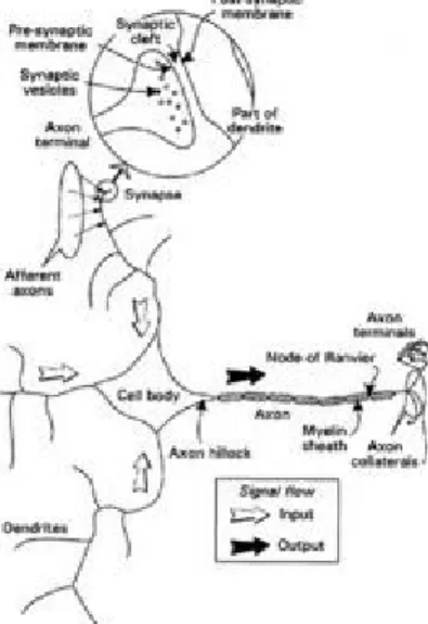
To flesh this out a little we first take a quick look at some basic neurobiology. The human brain consists of an estimated 1011 (100 billion) nerve cells or neurons, a highly stylized example of which is shown in Figure 1.1. Neurons communicate via electrical signals that are short-lived impulses or "spikes" in the voltage of the cell wall or membrane. The interneuron connections are mediated by electrochemical junctions called synapses, which are located on branches of the cell referred to as

dendrites. Each neuron typically receives many thousands of connections from

Figure 1.1 Essential components of a neuron shown in stylized form.

other neurons and is therefore constantly receiving a multitude of incoming signals, which eventually reach the cell body. Here, they are integrated or summed together in some way and, roughly speaking, if the resulting signal exceeds some threshold then the neuron will "fire" or generate a voltage impulse in response. This is then transmitted to other neurons via a branching fibre known as the axon.

(14)

It is this architecture and style of processing that we hope to incorporate in neural networks and, because of the emphasis on the importance of the interneuron connections, this type of system is sometimes referred to as being connectionist

and the study of this general approach as connectionism. This terminology is often the one encountered for neural networks in the context of psychologically inspired models of human cognitive function. However, we will use it quite generally to refer to neural networks without reference to any particular field of application.

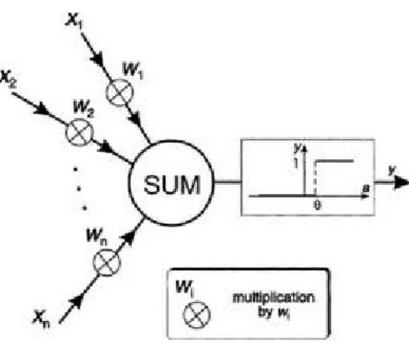
The artificial equivalents of biological neurons are the nodes or units in our preliminary definition and a prototypical example is shown in Figure 1.2. Synapses are modelled by a single number or weight so that each input is multiplied by a weight before being sent to the equivalent of the cell body. Here, the weighted signals are summed together by simple arithmetic addition to supply a node

activation. In the type of node shown in Figure 1.2—the so-called threshold logic unit (TLU)—the activation is then compared with a threshold; if the activation exceeds the threshold, the unit produces a high-valued output (conventionally "1"), otherwise it outputs zero. In the figure, the size of signals is represented by

(15)

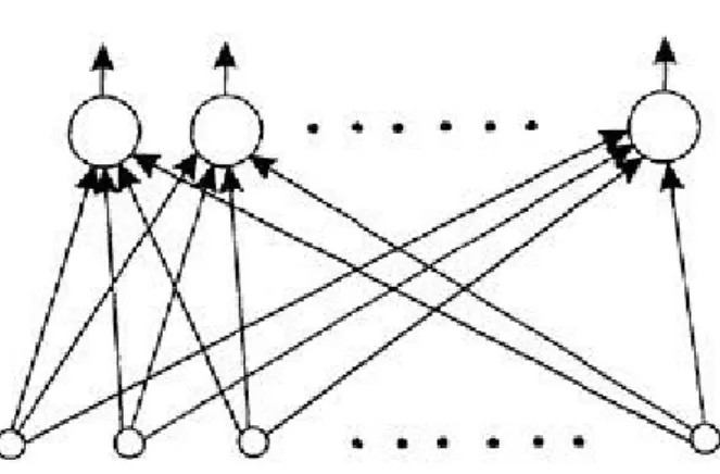
Figure 1.3 Simple example of neural network.

the width of their corresponding arrows, weights are shown by multiplication symbols in circles, and their values are supposed to be proportional to the symbol's size; only positive weights have been used. The TLU is the simplest (and historically the earliest (McCulloch & Pitts 1943)) model of an artificial neuron.

The term "network" will be used to refer to any system of artificial neurons. This may range from something as simple as a single node to a large collection of nodes in which each one is connected to every other node in the net. One type of network is shown in Figure 1.3. Each node is now shown by only a circle but weights are implicit on all connections. The nodes are arranged in a layered structure in which each signal emanates from an input and passes via two nodes before reaching an output beyond which it is no longer transformed. This feedforward structure is only one of several available and is typically used to place an input pattern into one of several classes according to the resulting pattern of outputs. For example, if the input consists of an encoding of the patterns of light and dark in an image of handwritten letters, the output layer (topmost in the figure) may contain 26 nodes— one for each letter of the alphabet—to flag which letter class the input character is from. This would be done by allocating one output node per class and requiring that only one such node fires whenever a pattern of the corresponding class is supplied at the input.

(16)

corresponding target. The process as a whole, including any ordering of pattern presentation, criteria for terminating the process, etc., constitutes the training algorithm.

(17)

1.2 Why study neural networks?

This question is pertinent here because, depending on one's motive, the study of connectionism can take place from differing perspectives. It also helps to know what questions we are trying to answer in order to avoid the kind of religious wars that sometimes break out when the words "connectionism" or "neural network" are mentioned.

Neural networks are often used for statistical analysis and data modelling, in which their role is perceived as an alternative to standard nonlinear regression or cluster analysis techniques (Cheng & Titterington 1994). Thus, they are typically used in problems that may be couched in terms of classification, or forecasting. Some examples include image and speech recognition, textual character recognition, and domains of human expertise such as medical diagnosis, geological survey for oil, and financial market indicator prediction. This type of problem also falls within the domain of classical artificial intelligence (AI) so that engineers and computer scientists see neural nets as offering a style of parallel distributed computing,

thereby providing an alternative to the conventional algorithmic techniques that have dominated in machine intelligence. This is a theme pursued further in the final chapter but, by way of a brief explanation of this term now, the parallelism refers to the fact that each node is conceived of as operating independently and concurrently (in parallel with) the others, and the "knowledge" in the network is distributed over the entire set of weights, rather than focused in a few memory locations as in a conventional computer. The practitioners in this area do not concern themselves with biological realism and are often motivated by the ease of implementing solutions in digital hardware or the efficiency and accuracy of particular techniques. Haykin (1994) gives a comprehensive survey of many neural network techniques from an engineering perspective.

Neuroscientists and psychologists are interested in nets as computational models of the animal brain developed by abstracting what are believed to be those properties of real nervous tissue that are essential for information processing. The artificial neurons that connectionist models use are often extremely simplified versions of their biological counterparts and many neuroscientists are sceptical about the ultimate power of these impoverished models, insisting that more detail is necessary to explain the brain's function. Only time will tell but, by drawing on knowledge about how real neurons are interconnected as local "circuits", substantial inroads have been made in modelling brain functionality. A good introduction to this programme of computational neuroscience is given by Churchland & Sejnowski (1992).

(18)

interest in nonlinear dynamical systems, statistical mechanics and automata theory.1 It is the job of applied mathematicians to discover and formalize the properties of new systems using tools previously employed in other areas of science. For example, there are strong links between a certain type of net (the Hopfield net—see Ch. 7) and magnetic systems known as spin glasses. The full mathematical apparatus for exploring these links is developed (alongside a series of concise summaries) by Amit (1989).

All these groups are asking different questions: neuroscientists want to know how animal brains work, engineers and computer scientists want to build intelligent machines and mathematicians want to understand the fundamental properties of networks as complex systems. Another (perhaps the largest) group of people are to be found in a variety of industrial and commercial areas and use neural networks to model and analyze large, poorly understood datasets that arise naturally in their workplace. It is therefore important to understand an author's perspective when reading the literature. Their common focal point is, however, neural networks and is potentially the basis for close collaboration. For example, biologists can usefully learn from computer scientists what computations are necessary to enable animals to solve particular problems, while engineers can make use of the solutions nature has devised so that they may be applied in an act of "reverse engineering".

(19)

1.3 Summary

Artificial neural networks may be thought of as simplified models of the networks of neurons that occur naturally in the animal brain. From the biological viewpoint the essential requirement for a neural network is that it should attempt to capture what we believe are the essential information processing features of the corresponding "real" network. For an engineer, this correspondence is not so important and the network offers an alternative form of parallel computing that might be more appropriate for solving the task in hand.

(20)

1.4 Notes

(21)

Chapter Two

Real and artificial neurons

(22)

2.1 Real neurons: a review

Neurons are not only enormously complex but also vary considerably in the details of their structure and function. We will therefore describe typical properties enjoyed by a majority of neurons and make the usual working assumption of connectionism that these provide for the bulk of their computational ability. Readers interested in finding out more may consult one of the many texts in neurophysiology; Thompson (1993) provides a good introductory text, while more comprehensive accounts are given by Kandel et al. (1991) and Kuffler et al. (1984).

A stereotypical neuron is shown in Figure 2.1, which should be compared with the simplified diagram in Figure 1.1. The cell body or soma contains the usual subcellular components or organelles to be found in most cells throughout the body (nucleus, mitochondria, Golgi body, etc.) but these are not shown in the diagram. Instead we focus on what differentiates neurons from other cells allowing the neuron to function as a signal processing device. This ability stems largely from the properties of the neuron's surface covering or membrane, which supports a wide variety of electrochemical processes. Morphologically the main difference lies in the set of fibres that emanate from the cell body. One of these fibres—the axon—is responsible for transmitting signals to other neurons and may therefore be considered the neuron output. All other fibres are dendrites, which carry signals from other neurons to the cell body, thereby acting as neural

Figure 2.1 Biological neuron.

(23)

axon may, however, branch into a set of collaterals allowing contact to be made with many other neurons. With respect to a particular neuron, other neurons that supply input are said to be afferent, while the given neuron's axonal output, regarded as a projection to other cells, is referred to as an efferent. Afferent axons are said to innervate a particular neuron and make contact with dendrites at the junctions called synapses. Here, the extremity of the axon, or axon terminal, comes into close proximity with a small part of the dendritic surface—the postsynaptic

membrane. There is a gap, the synoptic cleft, between the presynaptic axon terminal membrane and its postsynaptic counterpart, which is of the order of 20 nanometres (2×10-8m) wide. Only a few synapses are shown in Figure 2.1 for the sake of clarity but the reader should imagine a profusion of these located over all dendrites and also, possibly, the cell body. The detailed synaptic structure is shown in schematic form as an inset in the figure.

(24)

Figure 2.2 Action-potential propagation.

on the interplay between each of the ionic currents across the membrane and its mathematical description is complex. The details do not concern us here, but this example serves to illustrate the kind of simplification we will use when we model using artificial neurons; real axons are subject to complex, nonlinear dynamics but will be modelled as a passive output "wire". Many neurons have their axons sheathed in a fatty substance known as myelin, which serves to enable the more rapid conduction of action potentials. It is punctuated at approximately 1 mm intervals by small unmyelinated segments (nodes of Ranvier in Fig. 2.1), which act rather like "repeater stations" along a telephone cable.

We are now able to consider the passage of signals through a single neuron, starting with an action potential reaching an afferent axon terminal. These contain a chemical substance or neurotransmitter held within a large number of small

(25)

where it joins the soma. Concurrent with this are thousands of other synaptic events distributed over the neuron. These result in a plethora of PSPs, which are continually arriving at the axon hillock where they are summed together to produce a resultant membrane potential.

Each contributory PSP at the axon hillock exists for an extended time (order of milliseconds) before it eventually decays so that, if two PSPs arrive slightly out of synchrony, they may still interact in the summation process. On the other hand, suppose two synaptic events take place with one close to and another remote from the soma, by virtue of being at the end of a long dendritic branch. By the time the PSP from the distal (remote) synapse has reached the axon hillock, that originating close to the soma will have decayed. Thus, although the initiation of PSPs may take place in synchrony, they may not be effective in combining to generate action potentials. It is apparent, therefore, that a neuron sums or integrates its PSPs over both space and time. Substantial modelling effort—much of it pioneered by Rail (1957, 1959)—has gone into describing the conduction of PSPs along dendrites and their subsequent interaction although, as in the case of axons, connectionist models usually treat these as passive wires with no temporal characteristics.

The integrated PSP at the axon hillock will affect its membrane potential and, if this exceeds a certain threshold (typically about -50mV), an action potential is generated, which then propagates down the axon, along any collaterals, eventually reaching axon terminals resulting in a shower of synaptic events at neighbouring neurons "downstream" of our original cell. In reality the "threshold" is an emergent or meta-phenomenon resulting from the nonlinear nature of the Hodgkin-Huxley dynamics and, under certain conditions, it can be made to change. However, for many purposes it serves as a suitable high-level description of what actually occurs. After an action potential has been produced, the ionic metabolites used in its production have been depleted and there is a short refractory period during which, no matter what value the membrane potential takes, there can be no initiation of another action potential.

It is useful at this stage to summarize what we have learnt so far about the functionality of real neurons with an eye to the simplification required for modelling their artificial counterparts.

– Signals are transmitted between neurons by action potentials, which have a stereotypical profile and display an "all-or-nothing" character; there is no such thing as half an action potential.

(26)

– The PSPs may be excitatory or inhibitory.

– The PSPs are summed together at the axon hillock with the result expressed as its membrane potential.

– If this potential exceeds a threshold an action potential is initiated that proceeds along the axon.

Several things have been deliberately omitted here. First, the effect that synaptic structure can have on the value of the PSP. Factors that may play a role here include the type and availability of neurotransmitter, the postsynaptic receptors and synaptic geometry. Secondly, the spatio-temporal interdependencies of PSPs resulting from dendritic geometry whereby, for example, synapses that are remote from each other may not effectively combine. Finally, we have said nothing about t h e dynamics of action-potential generation and propagation. However, our summary will serve as a point of departure for defining the kind of artificial neurons described in this book. More biologically realistic models rely on solving Hodgkin-Huxley-type dynamics and modelling dendrites at the electrical circuit level; details of these methods can be found in the review compilation of Koch & Segev (1989).

2.1.1 Glossary of terms

Those terms in italics may be cross-referenced in this glossary.

action potential The stereotypical voltage spike that constitutes an active output from a neuron. They are propagated along the axon to other neurons.

afferent With respect to a particular neuron, an axon that impinges on (or

innervates) that neuron.

arbor Usually used in the context of a dendritic arbor—the tree-like structure associated with dendritic branching.

axon The fibre that emanates from the neuron cell body or soma and that conducts

action potentials to other neurons.

axon hillock The junction of the axon and cell body or soma. The place where

action potentials are initiated if the membrane potential exceeds a threshold.

(27)

axon terminal, which constitutes the presynaptic component of a synapse.

chemical binding The process in which a neurotransmitter joins chemically with a

receptor site thereby initiating a PSP.

collateral An axon may divide into many collateral branches allowing contact with many other neurons or many contacts with one neuron.

dendrite One of the branching fibres of a neuron, which convey input information via PSPs.

depolarization The membrane potential of the neuron has a negative resting or equilibrium value. Making this less negative leads to a depolarization. Sufficient depolarization at the axon hillock will give rise to an action potential.

efferent A neuron sends efferent axon collaterals to other neurons.

EPSP Excitatory Postsynaptic Potential. A PSP that acts to depolarize the neural membrane.

hyperpolarization The membrane potential of the neuron has a negative resting or equilibrium value. Making this more negative leads to a hyperpolarization and inhibits the action of EPSPs, which are trying to depolarize the membrane.

innervate Neuron A sending signals to neuron B is said to innervate neuron B.

IPSP Inhibitory Postsynaptic Potential. A PSP that acts to hyperpolarize the neural membrane.

membrane potential The voltage difference at any point across the neural membrane.

neurotransmitter The chemical substance that mediates synaptic activity by propagation across the synaptic cleft.

organelle Subcellular components that partake in metabolism, etc.

postsynaptic membrane That part of a synapse which is located on the dendrite

and consists of the dendritic membrane together with receptor sites.

potential difference The voltage difference across the cell membrane.

(28)

terminal.

PSP Postsynaptic Potential. The change in membrane potential brought about by activity at a synapse.

receptor sites The sites on the postsynaptic membrane to which molecules of

neurotransmitter bind. This binding initiates the generation of a PSP.

refractory period The shortest time interval between two action potentials.

soma The cell body.

synapse The site of physical and signal contact between neurons. On receipt of an

action potential at the axon terminal of a synapse, neurotransmitter is released into the synaptic cleft and propagates to the postsynaptic membrane. There it undergoes chemical binding with receptors, which, in turn, initiates the production of a postsynaptic potential (PSP).

(29)

2.2 Artificial neurons: the TLU

Our task is to try and model some of the ingredients in the list above. Our first attempt will result in the structure described informally in Section 1.1.

The "all-or-nothing" character of the action potential may be characterized by using a two-valued signal. Such signals are often referred to as binary or Boolean2 and conventionally take the values "0" and "1". Thus, if we have a node receiving n

input signals x₁, x₂,…, x_n, then these may only take on the values "0" or "1". In line with the remarks of the previous chapter, the modulatory effect of each synapse is encapsulated by simply multiplying the incoming signal with a weight value, where excitatory and inhibitory actions are modelled using positive and negative values respectively. We therefore have n weights w₁, w₂,…, w_n and form the n products

w₁x₁, w₂x₂,…, w_nx_n. Each product is now the analogue of a PSP and may be negative or positive, depending on the sign of the weight. They should now be combined in a process which is supposed to emulate that taking place at the axon hillock. This will be done by simply adding them together to produce the activation a (corresponding to the axon-hillock membrane potential) so that

(2.1)

As an example, consider a five-input unit with weights (0.5, 1.0, -1.0, -0.5, 1.2), that is w₁=0.5, w₂=1.0,…, w₅=1.2, and suppose this is presented with inputs (1, 1, 1, 0, 0) so that x₁=1, x₂=1,…, x₅=0. Using (2.1) the activation is given by

(30)

signals. This type of artificial neuron is known as a threshold logic unit (TLU) and was originally proposed by McCulloch and Pitts (McCulloch & Pitts 1943).

It is more convenient to represent the TLU functionality in a symbolic rather than a graphical form. We already have one form for the activation as supplied by (2.1). However, this may be written more compactly using a notation that makes use of the way we have written the weights and inputs. First, a word on

Figure 2.3 Activation-output threshold relation in graphical form.

Figure 2.4 TLU.

the notation is relevant here. The small numbers used in denoting the inputs and weights are referred to as subscripts. If we had written the numbers near the top (e.g. x1) they would have been superscripts and, quite generally, they are called

(31)

(2.2)

where E (upper case Greek sigma) denotes summation. The expressions above and below E denote the upper and lower limits of the summation and tell us that the index i runs from 1 to n. Sometimes the limits are omitted because they have been defined elsewhere and we simply indicate the summation index (in this case i) by writing it below the E.

The threshold relation for obtaining the output y may be written

(2.3)

(32)

2.3 Resilience to noise and hardware failure

Even with this simple neuron model we can illustrate two of the general properties of neural networks. Consider a two-input TLU with weights (0, 1) and threshold 0.5. Its response to all four possible input sets is shown in Table 2.1.

Now suppose that our hardware which implements the TLU is faulty so that the weights are not held at their true values and are encoded instead as (0.2, 0.8). The revised TLU functionality is given in Table 2.2. Notice that, although the activation has changed, the output is the same as that for the original TLU. This is because changes in the activation, as long as they don't cross the threshold, produce no change in output. Thus, the threshold function doesn't care whether the activation is just below or is very much less than ; it still outputs a 0. Similarly, it doesn't matter by how much the activation exceeds , the TLU always supplies a 1 as output.

This behaviour is characteristic of nonlinear systems. In a linear system, the output is proportionally related to the input: small/large changes in the input always produce corresponding small/large changes in the output. On the other hand, nonlinear relations do not obey a proportionality restraint so the magnitude of the change in output does not necessarily reflect that of the input. Thus, in our TLU example, the activation can change from 0 to 0.2 (a difference of 0.2) and make no difference to the output. If, however, it were to change from 0.49 to 0.51 (a difference of 0.02) the output would suddenly alter from 0 to 1.

(33)

if our hardware breaks down "slightly" the TLU may still function perfectly well as a result of its nonlinear functionality.

(34)

2.4 Non-binary signal communication

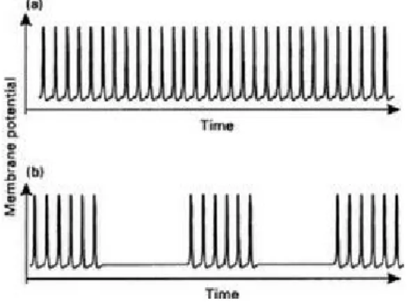
The signals dealt with so far (for both real and artificial neurons) have taken on only two values. In the case of real neurons these are the action-potential spiking voltage and the axon-membrane resting potential. For the TLUs they were conveniently labelled "1" and "0" respectively. Real neurons, however, are believed to encode their signal values in the patterns of action-potential firing rather than simply by the presence or absence of a single such pulse. Many characteristic patterns are observed (Conners & Gutnick 1990) of which two common examples are shown in Figure 2.5.

Part (a) shows a continuous stream of action-potential spikes while (b) shows

Figure 2.5 Neural firing patterns.

a pattern in which a series of pulses is followed by a quiescent period, with this sequence repeating itself indefinitely. A continuous stream as in (a) can be characterized by the frequency of occurrence of action potential in pulses per second and it is tempting to suppose that this is, in fact, the code being signalled by the neuron. This was convincingly demonstrated by Hartline (1934, 1940) for the optic neurons of the Horseshoe crab Limulus in which he showed that the rate of firing increased with the visual stimulus intensity. Although many neural codes are available (Bullock et al. 1977) the frequency code appears to be used in many instances.

(35)

effects of signal degradation. However, the use of a step function at the output limits the signals to be binary so that, when TLUs are connected in networks (and they are working properly), there is no possibility of continuously graded signals occurring. This may be overcome by "softening" the step function to a continuous "squashing" function so that the output y depends smoothly on the activation a. One convenient form for this is the logistic sigmoid (or sometimes simply "sigmoid") shown in Figure 2.6.

As a tends to large positive values the sigmoid tends to 1 but never actually reaches this value. Similarly it approaches—but never quite reaches—0 as a tends to large negative values. It is of no importance that the upper bound is not f_max, since we can simply multiply the sigmoid's value by f_max if we wish to interpret y as a real firing rate. The sigmoid is symmetric about the y-axis value of 0.5;

Figure 2.6 Example of squashing function—the sigmoid.

the corresponding value of the activation may be thought of as a reinterpretation of the threshold and is denoted by . The sigmoid function is conventionally designated by the Greek lower case sigma, , and finds mathematical expression according to the relation

(2.4)

(36)

be thought of as a special case. The reference to as a threshold then becomes more plausible as it takes on the role of the same parameter in the TLU.

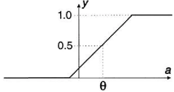
Artificial neurons or units that use the sigmoidal output relation are referred to as being of the semilinear type. The activation is still given by Equation (2.2) but now the output is given by (2.4). They form the bedrock of much work in neural nets since the smooth output function facilitates their mathematical description. The term "semilinear" comes from the fact that we may approximate the sigmoid by a continuous, piecewise-linear function, as shown in Figure 2.7. Over a significant region of interest, at intermediate values of the activation, the output function is a linear relation with non-zero slope.

As an alternative to using continuous or analogue signal values, we may emulate the real neuron and encode a signal as the frequency of the occurrence of a "1" in a pulse stream as shown in Figure 2.8.

Time is divided into discrete "slots" and each slot is filled with either a 0 (no pulse) or a 1 (pulse). The unit output is formed in exactly the same way as before but, instead of sending the value of the sigmoid function directly, we interpret it as the probability of emitting a pulse or "1". Processes that are governed by probabilistic laws are referred to as stochastic so that these nodes might be dubbed

stochastic semilinear units, and they produce signals quite close in general

Figure 2.7 Piecewise-linear approximation of sigmoid.

(37)

appearance to those of real neurons. How are units downstream that receive these signals supposed to interpret their inputs? They must now integrate over some number, N, of time slots. Thus, suppose that the afferent node is generating pulses with probability y. The expected value of the number of pulses over this time is yN

but, in general, the number actually produced, N₁, will not necessarily be equal to this. The best estimate a node receiving these signals can make is the fraction,

(38)

2.5 Introducing time

Although time reared its head in the last section, it appeared by the back door, as it were, and was not intrinsic to the dynamics of the unit—we could choose not to integrate, or, equivalently, set N=1. The way to model the temporal summation of PSPs at the axon hillock is to use the rate of change of the activation as the fundamental defining quantity, rather than the activation itself. A full treatment requires the use of a branch of mathematics known as the calculus but the resulting behaviour may be described in a reasonably straightforward way. We shall, however, adopt the calculus notation dx/dt, for the rate of change of a quantity x. It cannot be overemphasized that this is to be read as a single symbolic entity,

"dx/dt", and not as dx divided by dt. To avoid confusion with the previous notation it is necessary to introduce another symbol for the weighted sum of inputs, so we define

(2.5)

The rate of change of the activation, da/dt, is then defined by

(2.6)

where (alpha) and (beta) are positive constants. The first term gives rise to activation decay, while the second represents the input from the other units. As usual the output y is given by the sigmoid of the activation, y= (a). A unit like this is sometimes known as a leaky integrator for reasons that will become apparent shortly.

(39)

or da/dt= s where is a constant. Now suppose there is no inflow, but the outlet is working. The rate at which water leaves is directly proportional to the water pressure at the outlet, which is, in turn, proportional to the depth of water in the tank. Thus, the rate of water emission may be written as a litres per minute where is some constant. The water level is now decreasing so that its rate of change is now negative and we have da/dt=- a. If both hose and outlet are functioning then

da/dt is the sum of contributions from both, and its governing equation is just the same as that for the neural activation in (2.6). During the subsequent discussion it might be worth while referring back to this analogy if the reader has any doubts about what is taking place.

Figure 2.9 Water tank analogy for leaky integrators.

Returning to the neural model, the activation can be negative or positive (whereas the water level is always positive in the tank). Thus, on putting s=0, so that the unit has no external input, there are two cases:

(a) a>0. Then da/dt<0. That is, the rate of change is negative, signifying a decrease of a with time.

(b) a<0. Then da/dt>0. That is, the rate of change is positive, signifying an increase of a with time.

(40)

Figure 2.10 Activation decay in leaky integrator.

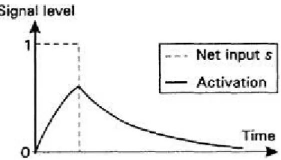
Suppose now that we start with activation zero and no input, and supply a constant input s=1 for a time t before withdrawing it again. The activation resulting from this is shown in Figure 2.11. The activation starts to increase but does so rather sluggishly. After s is taken down to zero, a decays in the way described above. If s

had been maintained long enough, then a would have eventually reached a constant value. To see what this is we put da/dt=0, since this is a statement of there being no rate of change of a, and a is constant at some equilibrium value a_eqm. Putting

da/dt=0 in (2.6) gives

(2.7)

that is, a constant fraction of s. If = then a_eqm=s. The speed at which a can respond to an input change may be characterized by the time taken to reach some fraction of a_eqm (0.75a_eqm, say) and is called the rise-time.

Figure 2.11 Input pulse to leaky integrator.

(41)

time to decay to its resting value in the interim, the peak value obtained this time is larger than before. Thus the two signals interact with each other and there is temporal summation or integration (the "integrator" part of the unit's name). In a TLU, the activation would, of course, just be equal to s. The value of the constants and govern the decay rate and rise-time respectively and, as they are increased, the decay rate increases and the rise-time falls. Keeping = and letting both become very large therefore allows a to rise and fall very quickly and to reach equilibrium at s. As these constants are increased further, the resulting behaviour of

a becomes indistinguishable from that of a TLU, which can therefore be thought of as a special case of the leaky integrator with very large constants , (and, of course, very steep sigmoid).

Leaky integrators find their main application in self-organizing nets (Ch. 8) . They have been studied extensively by Stephen Grossberg who provides a review in Grossberg (1988). What Grossberg calls the "additive STM model" is essentially the same as that developed here, but he also goes on to describe another—the "shunting STM" neuron—which is rather different.

This completes our first foray into the realm of artificial neurons. It is adequate for most of the material in the rest of this book but, to round out the story, Chapter 10 introduces some alternative structures.

(42)

2.6 Summary

The function of real neurons is extremely complex. However, the essential information processing attributes may be summarized as follows. A neuron receives input signals from many other (afferent) neurons. Each such signal is modulated (by the synaptic mechanism) from the voltage spike of an action potential into a continuously variable (graded) postsynaptic potential (PSP). PSPs are integrated by the dendritic arbors over both space (many synaptic inputs) and time (PSPs do not decay to zero instantaneously). PSPs may be excitatory or inhibitory and their integrated result is a change in the membrane potential at the axon hillock, which may serve to depolarize (excite or activate) or hyperpolarize (inhibit) the neuron. The dynamics of the membrane under these changes are complex but may be described in many instances by supposing that there is a membrane-potential threshold, beyond which an action potential is generated and below which no such event takes place. The train of action potentials constitutes the neural "output". They travel away from the cell body along the axon until they reach axon terminals (at synapses) upon which the cycle of events is initiated once again. Information is encoded in many ways in neurons but a common method is to make use of the frequency or rate of production of action potentials.

(43)

2.7 Notes

1. The millivolt (mV) is one-thousandth of a volt.

2. After George Boole who developed a formal logic with two values denoting "True" and "False".

(44)

Chapter Three

TLUs, linear separability and vectors

(45)

3.1 Geometric interpretation of TLU action

In summary, a TLU separates its input patterns into two categories according to its binary response ("0" or "1") to each pattern. These categories may be thought of as regions in a multidimensional space that are separated by the higher dimensional equivalent of a straight line or plane.

These ideas are now introduced step by step and in a way that should help put to rest any concerns about "higher dimensionality" and "multidimensional spaces".

3.1.1 Pattern classification and input space

Consider a two-input TLU with weights w₁=1, w₂=1 and threshold 1.5, as shown in Figure 3.1. The responses to the four possible Boolean inputs are shown i n Table 3.1. The TLU may be thought of as classifying its input patterns into two groups: those that give output "1" and those that give output "0". Each input pattern has two

components, x₁, x₂. We may therefore represent these patterns in a two-dimensional space as shown in Figure 3.2.

Each pattern determines a point in this so-called pattern space by using its

(46)

Figure 3.2 Two-input patterns in pattern space.

component values as space co-ordinates—just as grid references can locate points in physical space on a normal geographical map. In general, for n inputs, the pattern space will be n dimensional. Clearly, for n>3 the pattern space cannot be drawn or represented in physical space. This is not a problem. The key is that all relationships between patterns can be expressed either geometrically, as i n Figure 3.2, or algebraically using the notion of vectors. We can then gain insight into pattern relationships in two dimensions (2D), reformulate this in vector form and then simply carry over the results to higher dimensions. This process will become clearer after it has been put to use later. All the necessary tools for using vectors are introduced in this chapter; their appreciation will significantly increase any understanding of neural nets.

We now develop further the geometric representation of our two-input TLU.

3.1.2 The linear separation of classes

Since the critical condition for classification occurs when the activation equals the threshold, we will examine the geometric implication of this. For two inputs, equating and a gives

(3.1)

(47)

(3.2)

and dividing both sides by w₂ gives

(3.3)

This is of the general form

(3.4)

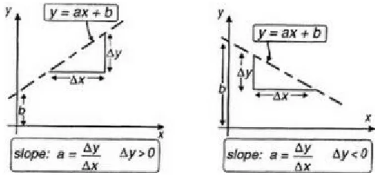
where a and b are constants. This equation describes a straight line with slope a

and intercept b on the x₂ axis. This is illustrated in Figure 3.3 where the graph of the equation y=ax+b has been plotted for two sets of values of a, b. In each case the slope is given by the change y that occurs in y when a positive change x is made in x (" " is Greek upper case delta and usually signifies a change in a

Figure 3.3 Straight line graphs.

(48)

increased, resulting in a negative slope.

For the TLU example, inserting the values of w₁, w₂, in (3.3) we obtain a=-1,

b=1.5 as shown in Figure 3.4, which also shows the output of the TLU for each pattern. The two classes of TLU output are separated by the line produced in this way so that the 1s (there is only one of them) and 0s lie on opposite sides of the line; we therefore talk of this as the decision line. Clearly, it is always possible to partition the two classes in 2D by drawing some kind of line—the point here is that the line is a straight one having no kinks or bends. It turns out that this is not just a fortuitous result made possible by our choice of weights and threshold. It holds true for any two-input TLU. This distinction is clearer in 3D where, quite generally, we can define a decision surface that may have to be highly convoluted but a TLU will necessarily be associated with a flat decision plane.

Figure 3.4 Decision line in two-input example.

Further, it is possible to generalize this result (in its algebraic form) to TLUs with an arbitrary number, n say, of inputs; that is, it is always possible to separate the two output classes of a TLU by the n-dimensional equivalent of a straight line in 2D or, in 3D, a plane. In n dimensions this is referred to as the decision hyperplane. (The "hyper-" is sometimes dropped even when n>3). Because TLUs are intimately related to linear relations like (3.3) (and their generalization) we say that TLUs are

linear classifiers and that their patterns are linearly separable. The converse of our result is also true: any binary classification that cannot be realized by a linear decision surface cannot be realized by a TLU.

(49)

3.2 Vectors

Vectors are usually introduced as representations of quantities that have magnitude and direction. For example, the velocity of the wind is defined by its speed and direction. On paper we may draw an arrow whose direction is the same as that of the wind and whose length is proportional to its speed. Such a representation is the basis for some of the displays on televised weather reports, and we can immediately see when there will be high winds, as these are associated with large arrows. A single vector is illustrated in Figure 3.5, which illustrates some notation.

Figure 3.5 A vector.

Vectors are usually denoted in printed text by bold face letters (e.g. v), but in writing them by hand we can't use bold characters and so make use of an underline as in v. The magnitude (or length) of v will be denoted by ||v|| but is also sometimes denoted by the same letter in italic face (e.g. v). In accordance with our geometric ideas a vector is now defined by the pair of numbers (||v||, ) where is the angle the vector makes with some reference direction. Vectors are to be distinguished from simple numbers or scalars, which have a value but no direction.

In order to generalize to higher dimensions, and to relate vectors to the ideas of pattern space, it is more convenient to describe vectors with respect to a rectangular or cartesian co-ordinate system like the one used for the TLU example in 2D. That is, we give the projected lengths of the vector onto two perpendicular axes as shown in Figure 3.6.

The vector is now described by the pair of numbers v₁, v₂. These numbers are its

components in the chosen co-ordinate system. Since they completely determine the vector we may think of the vector itself as a pair of component values and write

(50)

scalars (see below). To motivate the following technical material, we note that there are two vectors of immediate concern to us—the weight vector (w₁, w₂,…, w_n) and the input vector (x₁, x₂,…, x_n) for artificial neurons.

Figure 3.6 Vector components.

3.2.1 Vector addition and scalar multiplication

Multiplying a vector by a number (scalar) k simply changes the length of the vector by this factor so that if k=2, say, then we obtain a vector of twice the length. Multiplying by a negative number results in a reversal of vector direction and a change in length required by the number's magnitude—see Figure 3.7. In component terms, if a vector in 2D, v=(v₁, v₂), is multiplied by k, then the result1 v' has components (kv₁, kv₂). This can be seen in the right hand side of Figure 3.7 where the original vector v is shown stippled. Generalizing to n dimensions we define

vector multiplication by kv=(kv₁, kv₂,…, kv_n).

Geometrically, two vectors may be added in 2D by simply appending one to

(51)

Figure 3.8 Vector addition.

the end of the other as shown in Figure 3.8. Notice that a vector may be drawn anywhere in the space as long as its magnitude and direction are preserved. In terms of the components, if w=u+v, then w₁=u₁+v₁, w₂=u₂+v₂. This lends itself to generalization in n dimensions in a straightforward way. Thus, if u, v are now vectors in n dimensions with sum w, w=(u₁+v₁, u₂+v₂,…, u_n+v_n). Note that

u+v=v+u.

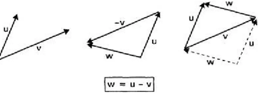
Vector subtraction is defined via a combination of addition and scalar multiplication so that we interpret u-v as u+(-1)v, giving the addition of u and a reversed copy of v (see Fig. 3.9). The left hand side of the figure shows the original vectors u and v. The construction for subtraction is shown in the centre and the right hand side shows how, by making use of the symmetry of the situation, the resulting vector w may be drawn as straddling u and v themselves.

Figure 3.9 Vector subtraction.

(52)

For our prototype in 2D, the length of a vector is just its geometrical length in the plane. In terms of its components, this is given by applying Pythagoras's theorem to the triangle shown in Figure 3.10, so that

(3.5)

In n dimensions, the length is defined by the natural extension of this, so that

(3.6)

where the exponent of outside the square brackets is a convenient way of denoting the operation of square root.

Figure 3.10 Obtaining the length of a vector.

3.2.3 Comparing vectors—the inner product

(53)

this. This section relies on the trigonometric function known as the cosine and so, for those readers who may not be familiar with this, it is described in an appendix.

Inner product—geometric form

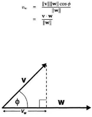
Suppose two vectors v and w are separated by an angle ø. Define the inner product

v·w of the two vectors by the product of their lengths and the cosine of ø; that is,

(3.7)

This is pronounced "v dot w" and is also known as the scalar product since its result is a number (rather than another vector). Note that v·w=w·v.

What is the significance of this definition? Essentially (as promised) it tells us something about the way two vectors are aligned with each other, which follows from the properties of the cosine function. To see this, fix w but allow v to vary its direction (but not its lengths) as shown in Figure 3.11. Then, if the lengths are fixed,

v·w can only depend on cosø. When 0<ø<90°, the cosine is positive and so too, therefore, is the inner product. However, as the angle approaches 90°, the cosine diminishes and eventually reaches zero. The inner product follows in sympathy with this and, when the two vectors are at right angles they are said to be

orthogonal with v·w=0. Thus, if the vectors are well aligned or point in roughly the same direction, the inner product is close to its largest positive value of ||v|| ||w||. As they move apart (in the angular sense) their inner product decreases until it is zero when they are orthogonal. As ø becomes greater than 90°, the cosine becomes progressively more negative until it reaches -1. Thus, ||v|| ||w|| also behaves in this way until, when ø=180°, it takes on its largest negative value of -||v|| ||w||. Thus, if the vectors are pointing in roughly opposite directions, they will have a relatively large negative inner product.

(54)

Note that we only need to think of angles in the range 0<ø<180° because a value of

ø between 180° and 360° is equivalent to an angle given by 360-ø.

Inner product—algebraic form

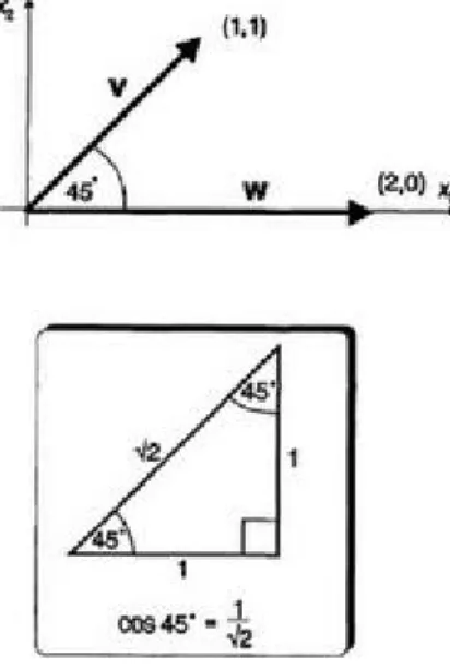
Consider the vectors v=(1, 1) and w=(0, 2) shown in Figure 3.12 where the angle between them is 45°. An inset in the figure shows a right-angled triangle with its other angles equal to 45°. The hypotenuse, h, has been calculated from Pythagoras's

theorem to be and, from the definition of the cosine (A.1), it can then

be seen that . To find the inner product

Figure 3.12 Vectors at 45°.

of the two vectors in Figure 3.12, we note that so that

. We now introduce an equivalent, algebraic definition of the inner product that lends itself to generalization in n dimensions.

Consider the quantity v O w defined in 2D by

(3.8)

(55)

occurrence resulting from the particular choice of numbers in our example. It is a general result (Rumelhart et al. 1986b) (which will not be proved here) and it means that we may write v·w=v₁w₁+v₂w₂ for any vectors v, w in 2D. The form in (3.8) immediately lends itself to generalization in n dimensions so that we define the dot product of two n-dimensional vectors v, w as

(3.9)

We shall interpret the value obtained in this way just as we did in 2D. Thus, if it is positive then the two vectors are, in some sense, roughly "lined up" with each other, if it is negative then they are "pointing away from" each other and, if it is zero, the vectors are at "right angles". No attempt should be made to visualize this i n n dimensions; rather, think of its analogue in 2D as a schematic or cartoon representation of what is happening. The situation is a little like using pictures in 2D to represent scenes in 3D—the picture is not identical to the objects it depicts in 3D, but it may help us think about their geometrical properties.

Finally, what happens if v=w? Then we have

(3.10)

so that the square length of vector is the same as the inner product of the vector with itself.

Vector projection

(56)

(3.11)

(57)

3.3 TLUs and linear separability revisited

Our discussion of vectors was motivated by the desire to prove that the connection between TLUs and linear separability is a universal one, independent of the dimensionality of the pattern space. We are now in a position to show this, drawing on the ideas developed in the previous section. Using the definition of the inner product (3.9) the activation a of an n-input TLU may now be expressed as

(3.12)

The vector equivalent to (3.1) now becomes

(3.13)

As in the example in 2D, we expect deviations either side of those x that satisfy this relation to result in different output for the TLU. We now formalize what is meant by "either side" a little more carefully. Our strategy is to examine the case in 2D geometrically to gain insight and then, by describing it algebraically, to generalize to n dimensions.

In general, for an arbitrary x, the projection of x onto w is given by

(3.14)

If, however, we impose the constraint implied by (3.13), we have

(58)

So, assuming w and are constant, the projection x_w is constant and, in 2D, x must actually lie along the perpendicular to the weight vector, shown as a dashed line in Figure 3.14. Therefore, in 2D, the relation w·x= defines a straight line. However, since we have used algebraic expressions that are valid in n dimensions throughout, we can generalize and use this to define the n-dimensional equivalent

Figure 3.14 Projection of x as decision line.

of a straight line—a hyperplane—which is perpendicular to the weight vector w. When x lies on the hyperplane, w·x= , and the TLU output rule states that y=1; it remains to see what happens on each side of the line.

Suppose first that x_w> /||w||; then the projection is longer than that in Figure 3.14 and x must lie in region A (shown by the shading). Comparison of (3.14) and (3.15) shows that, in this case, w·x> , and so y=1. Conversely, if x_w< /||w||, the projection is shorter than that in Figure 3.14 and x must lie in region B. The implication is now that w·x< , and so y=0. The diagram can only show part of each region and it should be understood that they are, in fact, of infinite extent so that any point in the pattern space is either in A or B. Again these results are quite general and are independent of the number n of TLU inputs.

To summarize: we have proved two things:

(a) The relation w·x= defines a hyperplane (n-dimensional "straight line") in pattern space which is perpendicular to the weight vector. That is, any vector wholly within this plane is orthogonal to w.

(59)

To recap on some points originally made in Section 3.1.2, the hyperplane is the decision surface for the TLU. Since this surface is the n-dimensional version of a straight line the TLU is a linear classifier. If patterns cannot be separated by a hyperplane then they cannot be classified with a TLU.

One assumption has been made throughout the above that should now be made explicit. Thus, Figure 3.14 shows a positive projection x_w, which implies a positive threshold. For a negative threshold , the projection constraint (3.15) now implies that x_w<0, since ||w|| is always positive. Therefore w·x<0 for

Figure 3.15 Projection with negative threshold.

(60)