Software effort estimation
CHAPTERObjectives
• Avoid the dangers of unrealistic estimates;
• Understand the range of estimating methods that can be used; • Estimate project using a bottom-up approach;
• Count the function points and object points for a system • Estimate the effort needed to implement software using a • Estimate the effort needed to implement software using a
procedural programming language;
Software effort estimation
5.1 Introduction
Definition of successful project:
“on time and within budget and with the required quality.” “on time and within budget and with the required quality.”
•
Novel applications of software;
•
Changing technology;
•
Lack of homogeneity of project experience
Software effort estimation
5.1 Introduction
Select Project
0
Identify project scope and objective
1 Identify project
infrastructure
2
Identify the products and activities
4 Estimate effort for activity 5 Identify activity risks 6 Analyze project characteristics 3
For each activity Lower level detail
Review
Allocate resources
7
Review/publicize plan
8
Lower level planning
10
Execute plan
9
Software effort estimation
5.1 Introduction
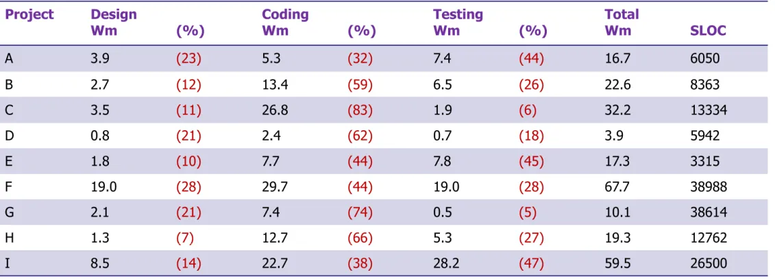
Table 5.1: Some project data – effort in work months
Project Design
Wm (%) CodingWm (%) TestingWm (%) TotalWm SLOC
A 3.9 (23) 5.3 (32) 7.4 (44) 16.7 6050
B 2.7 (12) 13.4 (59) 6.5 (26) 22.6 8363
C 3.5 (11) 26.8 (83) 1.9 (6) 32.2 13334
D 0.8 (21) 2.4 (62) 0.7 (18) 3.9 5942
E 1.8 (10) 7.7 (44) 7.8 (45) 17.3 3315
F 19.0 (28) 29.7 (44) 19.0 (28) 67.7 38988
G 2.1 (21) 7.4 (74) 0.5 (5) 10.1 38614
H 1.3 (7) 12.7 (66) 5.3 (27) 19.3 12762
H 1.3 (7) 12.7 (66) 5.3 (27) 19.3 12762
I 8.5 (14) 22.7 (38) 28.2 (47) 59.5 26500
Software effort estimation
5.1 Introduction
Subjective nature of estimating
•
Underestimate
•
Underestimate
•
Overestimate
Political implications
Different groups within an organization
Software effort estimation
5.2 Where are estimates done?
•
Strategic planning
•
Strategic planning
•
Feasibility study
•
System specification
•
Evaluation of suppliers
’
proposals
•
Project planning
Software effort estimation
5.3 Problem with over- and under-estimates
Parkinson
’
s Law
Work expands to fill the time available
Brooks
’
Law
Software effort estimation
5.3 Problem with over- and under-estimates
Under-estimate
• Not be completed on time or to cost;
• Implement in a shorter time than project with more generous estimate;
• The danger is the effect on quality;
Software effort estimation
5.4 The basis for software estimating
1. The need for historical data
1. The need for historical data
• It is impossible to calculate directly the actual cost
or time required to implement the project.
• Software measurement : source line of code
2. Measure of work
• Software measurement : source line of code
(SLOC) or thousands of line of code (KLOC).
Software effort estimation
5.5 Software effort estimation techniques
Algorithmic models
Expert judgment
Analogy
Parkinson
Price to win
A model is developed using historical cost
information which relates some software metric (usually its size) to the project cost. An estimate is made of that metric and model predicts the One or more experts on the software development
techniques to be used and on the application domain are consulted.
This technique is applicable when other projects in the same application domain
have been completed.The effort is determined byavailable resources rather than by objectiveThe estimated effort
Top-down
Bottom-up
and model predicts the effort required.
than by objective assessment.
The estimated effort
depends on the customer’s budget and not on the
software functionality.
Estimates are made on the basis of the logical function
Software effort estimation
5.5 Software effort estimation techniques
Bottom-up estimating
The estimator breaks the project into its component tasks and then estimates how much effort will be required to carry out this task.
With a large project, the process of breaking down into tasks would be a repetitive one: each task would be
analyzed into its component sub-tasks and these in turn would be further analyzed.
would be further analyzed.
This is repeated until you get to components that can be executed by a single person in about a week or two.
Software effort estimation
5.5 Software effort estimation techniques
The top-down approach and parametric models
• The top-down approach is normally associated with parametric • The top-down approach is normally associated with parametric
models.
• Form of parametric models’ formulation:
Effort = (system size) X (productivity rate)
The top-down and bottom-up approaches are not mutually exclusive. Project The top-down and bottom-up approaches are not mutually exclusive. Project managers will probably try to get a number of different estimates from
Software effort estimation
5.5 Software effort estimation techniques
The top-down approach and parametric models
Example Example
Software effort estimation
5.6 Expert judgement
Software effort estimation
5.7 Estimating by analogy
• Case-based reasoning;
• Estimator seeks out project that have been completed –
“Source cases”;
• That has been similar characteristics to the new project –
“Target cases”;
• The effort that has been recorded for the matching source case can then be used as a base estimate for the target;
• The estimator should then try to identify any differences
Software effort estimation
5.7 Estimating by analogy
The Euclidean distance is calculated:
2 2
1
1
sp
...
tp
nsp
ntp
distance =
Software effort estimation
5.7 Estimating by analogy
Example 5.1
The new project is known to require 7 inputs and 15 outputs. One of the past cases, project A, has 8 inputs and 17 outputs. The Euclidean distance between source and the target is =
Project B has 5 inputs and 10 outputs. What would be the Euclidean
Software effort estimation
Summary
Methodology Description
Analogy (Comparative)
Bottom-up (Grass Roots)
Top-down
Expert Judgment
Compare project with past similar projects
Individuals assess components, then component estimates are summed to obtain total estimate.
Project partitioned into lower level components & life cycle phases beginning at highest level
Consult with one or more experts.
Expert Judgment
Parametric (Algorithm)
Consult with one or more experts.
Software effort estimation
Summary
Methodology Advantages Analogy Bottom-up Top-downEstimates are based on actual experience.
Accurate estimates are possible because of detailed basis for estimate; also promotes individual
responsibility, supports project tracking.
More applicable to early project estimates. Considers system level activities,
faster, easier to implement.
Expert Judgment
Parametric
faster, easier to implement.
Little or no historical data are needed; good for new or unique projects.
Software effort estimation
Summary
Methodology
Analogy
Disadvantages
Truly similar projects must exist.
Analogy
Bottom-up
Top-down
Truly similar projects must exist.
• Methods are time-consuming.
• Detailed data needed may not be available, especially early in a program.
• Integration costs may be disregarded. • Process is costly
• Less accurate than other methods,
• tends to overlook lower-level components,
Top-down
Expert Judgment
• tends to overlook lower-level components, • provides little detail.
Software effort estimation
5.8 Albrecht function point analysis
The basis of function point analysis is that computer-based information systems comprise five major components, or external user types in Albrecht’s terminology, that are of benefit to the users: user types in Albrecht’s terminology, that are of benefit to the users:
External input types
External output types
Logical internal file types
Logical internal file types
External interface file types
Software effort estimation
5.8 Albrecht function point analysis
Case Study Examples: Assessing the complexity of a logical internal file
Table 5.2: Albrecht complexity multipliers
Multiplier
Low Average High
External user type
External input type External output type
3 4 6
4 5 7
External output type
Logical internal file type External interface file type
4 5 7
7 10 15
5 7 10
Software effort estimation
5.8 Albrecht function point analysis
Software effort estimation
5.8 Albrecht function point analysis
Complexity Tables: Albrecht Function point
External Input Table (EI) Shared EO and EQ Table
External Input Table (EI) Shared EO and EQ Table
Software effort estimation
5.8 Albrecht function point analysis
Complexity Tables: Albrecht Function point
Software effort estimation
5.8 Albrecht function point analysis
Level of selected software languages relative to Assembler language
Language Ratio-source : Executable
Assembler 1 : 1
C 1 : 1.5
COBOL 1 : 3
FORTRAN 1 : 3
PASCAL 1 : 3.5
RPG 1 : 4
RPG 1 : 4
PL/1 1 : 4
BASIC 1 : 5
Software effort estimation
5.8 Function points
Software effort estimation
Software effort estimation
5.9 Function points Mark II
The ‘Mark II’ label implies an improvement and replacement of the Albrecht method.
The information processing size is initially measured in
Software effort estimation
5.9 Function points Mark II
For each transaction the UFPs are calculated:
Wi x (number of input data element types) +
W x (number of entity types referenced) +
We x (number of entity types referenced) +
Wo x (number of output data element types)
Here, W is weightings that might be derived by asking developers what proportion of effort has been spent in previous projects developing those parts of the software that deal with processing inputs, assessing, and modifying stored data and processing outputs.
Data Store
Process
From Input Return
Software effort estimation
5.9 Function points Mark II
Case study Example: Calculating Mark II function points
• Two entity types – Invoice and CashReceipt • Two entity types – Invoice and CashReceipt
• Data elements – InvoiceNumber, DateReceived, CashReceived
• Output – error message
The unadjusted function points, using the industry average weightings, for this transaction would therefore be:
Software effort estimation
5.9 Function points Mark II
Example 5.7
The IOE maintenance group accounts subsystem for which Amanda is
• Customer account number • Customer Name
• Address • Postcode
• Customer Type
• Statement production date
The IOE maintenance group accounts subsystem for which Amanda is responsible will have a transaction which sets up details of new group account customers. The operator will input:
• Statement production date
Software effort estimation
5.9 Function points Mark II
The original Albrecht FP method identified 14 technical complexity adjustment factors – Mark II FPs identify five more factors:
• Interfaces to other applications;
• Special security features;
• Direct access for third parties;
• User training features;
• Documentation requirements.
Software effort estimation
5.9 Function points Mark II
If you have figures for the effort expended on past projects and also the system size in FPs, you should be able to work out a productivity rate, that is:
rate, that is:
Productivity = size / effort.
For new projects, the function points can be counted and then the effort can be projected using the productivity rate derived above:
Effort = size / productivity.
A more sophisticated way of doing this would be by using the
Software effort estimation
5.10 COSMIC Full Function Points
Common Software Measurement Consortium – Full Function Point
Full function point (FFP) method has its origins in the work of two interlinked research group.
interlinked research group.
COSMIC requires the analyst to break down the system architecture into a hierarchy of software layers.
Data groups can be moved about in four ways:
Entries (E)
Exits (X)
Reads (R)
Writes (W).
Software effort estimation
5.10 Object points
If you are building a system using a high level application building tool – object-oriented techniques, the approach uses counts of the screens, reports, and 3GL components that an counts of the screens, reports, and 3GL components that an application might possess – it is these that are referred to as
objects.
Each object has to be classified as one of the following:
Simple;
Medium;
Software effort estimation
5.10 Object points
Software effort estimation
5.10 Object points
Object Type Simple Medium Difficult
Complexity weighting
Object Type Simple Medium Difficult
Screen 1 2 3
Report 2 5 8
3GL
Component - - 10
Software effort estimation
5.10 Object points
If application containing 840 object points, 20% can be supplied by using existing components, then the adjusted new object points (NOP) score would be:
(NOP) score would be:
NOP = 840 x (100 – 20)/100 = 672
Productivity rate (PROD) has to be identified. An estimate of the
person-months needed to carry out the project is then calculated by dividing PROD into NOP.
Given 672 new object points and a development environment where Given 672 new object points and a development environment where productivity was nominal, then estimated effort for the project would be:
672/13 = 52 months.
Software effort estimation
5.11 A procedural code-oriented approach
1. Envisage the number and type of programs in
1. Envisage the number and type of programs in
the final system
2. Estimate the SLOC of each identified program
3. Estimate the work content, taking into account
complexity and technical difficulty
Software effort estimation
5.12 COCOMO : a parametric model
The COCOMO Model ( Barry Boehm 1981):
The COnstructive COst MOdel ( COCOMO) is an example of The COnstructive COst MOdel ( COCOMO) is an example of regression models used for estimating software cost and effort. These methods use a basic formula with parameters that are determined via a historical database and current project characteristics.
Software effort estimation
5.12 COCOMO : a parametric model
COCOMO (Constructive Cost Model) is often referred to in the literature on software project management, particularly in literature on software project management, particularly in connection with software estimating. The term COCOMO really refers to a group of models.
The basic model was built around the equation:
effort = c x sizek
Software effort estimation
5.12 COCOMO : a parametric model (ADD)
Small Projects:
Measurements of small to moderate projects resulted in a model of the following form:
EFFORT = a * SIZE + b
Here, the magnitude of the effort is a linear function of the size of the project ( Number of Lines of Code, usually ). This model holds up until a certain point, usually for projects that can be reasonably accomplished by small teams of two or three people. By increasing the size of the project, the above model becomes less and less accurate an the need for a new model increases.
Large Projects:
Projects requiring teams of more than three or so people tend to behave in the following Projects requiring teams of more than three or so people tend to behave in the following way:
EFFORT = a * SIZE b
Here, the size of the project is scaled exponentially, therefore as a product increases in size, the effort to produce the product grows more than linearly ( for b >= 1 ). It means that if we try to
Software effort estimation
5.12 COCOMO : a parametric model
The Organic Mode
Software developed “in house”
Software developed “in house”
Experienced developers
Requires small developer teams
Small communication overhead
Stable development environment
Stable development environment
Software effort estimation
5.12 COCOMO : a parametric model
Semi-Detached Mode
Developers have an intermediate level of experience
Developers have an intermediate level of experience
with related systems.
Mixture of experienced and unexperienced
developers.
Team can have experience relative only for some
project aspects.
project aspects.
Size extends up 300 KDSI
Software effort estimation
5.12 COCOMO : a parametric model
Embedded Mode
Projects developed within tight constraints.
Product must operate within (embedded in) a
strongly coupled complex of hardware, software
and operational procedures.
High cost on changing parts.
High cost on changing parts.
Software effort estimation
5.12 COCOMO : a parametric model
C
K
•
Organic Mode
•
Embedded Mode
•
Semi-detached Mode
2.4
1.05
3.6
1.20
3.0
1.12
Software effort estimation
5.12 COCOMO : a parametric model
The nominal estimate is then adjusted by a development effort multiplier (dem):
pm
= pm
x dem
pm
est= pm
nomx dem
Where dem is calculated by taking into account multipliers based on the effort drivers in Table 5.11
The effect of analyst capability: ACAP Very Low 1.46
Software effort estimation
5.12 COCOMO : a parametric model
Driver type Code Cost driver
Product attribute RELY Required software reliability
DATA Database size
DATA Database size
CPLX Product complexity
Computer attribute TIME Execution time constraints
STOR Main storage constraints VIRT Virtual machine volatility TURN Computer turn around time
Personnel attribute ACAP Analyst capability
AEXP Application experience AEXP Application experience PCAP Programmer capability
VEXP Virtual machine experience (OS)
LEXP Programming language experience
Project attribute MODP Use of modern programming practice
Software effort estimation
5.12 COCOMO : a parametric model
Attribute Very low Low Nominal High Very high
ACAP 1.46 1.19 1.00 0.86 0.71
ACAP 1.46 1.19 1.00 0.86 0.71
AEXP 1.29 1.13 1.00 0.91 0.82
PCAP 1.42 1.17 1.00 0.80 0.70
VEXP 1.21 1.10 1.00 0.90
-Software effort estimation
5.12 COCOMO : a parametric model
COCOMO II has been designed to accommodate this by having models for three different stages.
Application composition
Early design
Software effort estimation
Software effort estimation
5.12 COCOMO II : a parametric model
Software effort estimation
5.12 COCOMO II : a parametric model
To estimate the effort for application composition, the counting of object points, which were described earlier, is recommended by the
developers of COCOMO II. developers of COCOMO II.
At the early design stage, FPs are recommended as the way of gauging a basic system size. An FP count might be converted to a SLOC equivalent by multiplying the FPs by a factor for the programming
language that is to be used.
The following model can then be used to calculate an estimate of person-months: sf
em
em
em
size
A
pm
A
size
sf
em
em
...
em
npm
1
2
...
Software effort estimation
5.12 COCOMO II : a parametric model
Very Low Low Nominal High Very High
Effort Adjustment Factor (EAF)
Very Low Low Nominal High Very High 1. Product Distribution
- Software Reliability 0.75 0.88 1.00 1.15 1.40
- Database Size 0.94 0.94 1.00 1.08 1.16
- Product Complexity 0.70 0.85 1.00 1.15 1.30
2. Computer Distribution
- Execute time constraints 1.00 1.00 1.00 1.11 1.30
- Main storage constraints 1.00 1.00 1.00 1.06 1.21
- Virtual machine volitility 0.87 0.87 1.00 1.15 1.30
- Computer turnaround time 0.87 0.87 1.00 1.07 1.15
3. Personnel Distribution
- Analyst Capability 1.46 1.19 1.00 0.86 0.71
- Analyst Capability 1.46 1.19 1.00 0.86 0.71
- Applications experience 1.29 1.13 1.00 0.91 0.82
- Programmer capability 1.42 1.17 1.00 0.86 0.70
- Virtual machine experience 1.21 1.10 1.00 0.90 0.90
- Programming Language experience 1.14 1.07 1.00 0.95 0.95
4. Project attributes
- Use of modern programming practice 1.24 1.10 1.00 0.91 0.82
- Use of software tools 1.24 1.10 1.00 0.91 0.83
Software effort estimation
5.12 COCOMO II : a parametric model
The qualities that govern the exponent driver used to calculate the 5 scale factors are listed below:
Precedentedness
Development flexibility
Architecture/risk resolution
Team cohesion
Team cohesion
Software effort estimation
5.12 COCOMO II : a parametric model
COCOMO II Effort Equation
The COCOMO II model makes its estimates of required effort (measured in Person-Months – PM) based primarily on your estimate of the software project's size (as measured in
– PM) based primarily on your estimate of the software project's size (as measured in thousands of SLOC, KSLOC)):
Where
EAF is the Effort Adjustment Factor derived from the Cost Drivers
E is an exponent derived from the five Scale Drivers
Software effort estimation
5.12 COCOMO II : a parametric model
COCOMO II Schedule Equation
The COCOMO II schedule equation predicts the number of months required to complete your software project. The duration of a project is based on the effort predicted by the your software project. The duration of a project is based on the effort predicted by the effort equation:
Where
Effort is the effort from the COCOMO II effort equation
SE is the schedule equation exponent derived from the five Scale Drivers
Duration = 2.5 (Effort)SE
Software effort estimation
5.12 COCOMO II : Example
Consider a database system needed for an office automation project. The requirements document shows 4 modules needed. The project is judged to be ORGANIC
to be ORGANIC
Sizes are estimated as follows:
data entry 0.6 KDSI data update 0.6 KDSI query 0.8 KDSI report gen. 1.0 KDSI
The manager rates project details as follows: The manager rates project details as follows:
Complexity (HIGH) EAF = 1.15 Storage (HIGH) EAF = 1.06
Software effort estimation
5.12 COCOMO II : Example
PROJECT SIZE = 0.6 + 0.6 + 0.8 + 1.0 = 3.0 KDSI
EAF = 1.15 x 1.06 x 1.13 x 1.17 = 1.61
Person Months for the project:
PM = 1.61 x 3.2 x (3.0)1.05
PM = 1.61 x 3.2 x 3.17 PM = 16.33
DURATION DURATION
DURATION = 2.5 x EFFORT 0.38
DURATION = 2.5 x (16.33)0.38
Software effort estimation
5.12 COCOMO II : Example
Duration
Effort
Staffing
How Many people to hire ?
Staffing = 16.33 pm / 7.23 months = 2.26 persons
3 team members needed
Software effort estimation
5.13 Conclusion
To summarize some key points:
Estimates are really management targets
Estimates are really management targets
Collect as much information about previous projects as possible
Use more than one method of estimating
Top-down approaches will be used at the earlier stages of project planning
while bottom-up approaches will be more prominent later on
Be careful about using other people’s historical productivity data as a basis
for your estimates, especially if it comes from a different environment