FHSST Mathematics for Grade 10 - 12 - Free Computer, Programming, Mathematics, Technical Books, Lecture Notes and Tutorials

(1)

FHSST Authors

The Free High School Science Texts:

Textbooks for High School Students

Studying the Sciences

Mathematics

Grades 10 - 12

(2)

(3)

Permission is granted to copy, distribute and/or modify this document under the terms of the GNU Free Documentation License, Version 1.2 or any later version published by the Free Software Foundation; with no Invariant Sections, no Front-Cover Texts, and no Back-Front-Cover Texts. A copy of the license is included in the section entitled “GNU Free Documentation License”.

STOP!!!!

Did you notice the FREEDOMS we’ve granted you?

Our copyright license is

different!

It grants freedoms

rather than just imposing restrictions like all those other

textbooks you probably own or use.

• We know people copy textbooks illegally but we would LOVE it if you copied

our’s - go ahead copy to your hearts content,

legally!

• Publishers revenue is generated by controlling the market, we don’t want any

money, go ahead, distribute our books far and wide - we DARE you!

• Ever wanted to change your textbook? Of course you have! Go ahead change

ours, make your own version, get your friends together, rip it apart and put

it back together the way you like it. That’s what we really want!

• Copy, modify, adapt, enhance, share, critique, adore, and contextualise. Do it

all, do it with your colleagues, your friends or alone but get involved! Together

we can overcome the challenges our complex and diverse country presents.

• So what is the catch? The only thing you can’t do is take this book, make

a few changes and then tell others that they can’t do the same with your

changes. It’s share and share-alike and we know you’ll agree that is only fair.

(4)

(5)

FHSST Core Team

Mark Horner ; Samuel Halliday ; Sarah Blyth ; Rory Adams ; Spencer Wheaton

FHSST Editors

Jaynie Padayachee ; Joanne Boulle ; Diana Mulcahy ; Annette Nell ; Ren´e Toerien ; Donovan Whitfield

FHSST Contributors

Rory Adams ; Prashant Arora ; Richard Baxter ; Dr. Sarah Blyth ; Sebastian Bodenstein ; Graeme Broster ; Richard Case ; Brett Cocks ; Tim Crombie ; Dr. Anne Dabrowski ; Laura

Daniels ; Sean Dobbs ; Fernando Durrell ; Dr. Dan Dwyer ; Frans van Eeden ; Giovanni Franzoni ; Ingrid von Glehn ; Tamara von Glehn ; Lindsay Glesener ; Dr. Vanessa Godfrey ; Dr. Johan Gonzalez ; Hemant Gopal ; Umeshree Govender ; Heather Gray ; Lynn Greeff ; Dr. Tom Gutierrez ; Brooke Haag ; Kate Hadley ; Dr. Sam Halliday ; Asheena Hanuman ; Neil Hart ;

Nicholas Hatcher ; Dr. Mark Horner ; Mfandaidza Hove ; Robert Hovden ; Jennifer Hsieh ; Clare Johnson ; Luke Jordan ; Tana Joseph ; Dr. Jennifer Klay ; Lara Kruger ; Sihle Kubheka ;

Andrew Kubik ; Dr. Marco van Leeuwen ; Dr. Anton Machacek ; Dr. Komal Maheshwari ; Kosma von Maltitz ; Nicole Masureik ; John Mathew ; JoEllen McBride ; Nikolai Meures ; Riana Meyer ; Jenny Miller ; Abdul Mirza ; Asogan Moodaly ; Jothi Moodley ; Nolene Naidu ;

Tyrone Negus ; Thomas O’Donnell ; Dr. Markus Oldenburg ; Dr. Jaynie Padayachee ; Nicolette Pekeur ; Sirika Pillay ; Jacques Plaut ; Andrea Prinsloo ; Joseph Raimondo ; Sanya Rajani ; Prof. Sergey Rakityansky ; Alastair Ramlakan ; Razvan Remsing ; Max Richter ; Sean

Riddle ; Evan Robinson ; Dr. Andrew Rose ; Bianca Ruddy ; Katie Russell ; Duncan Scott ; Helen Seals ; Ian Sherratt ; Roger Sieloff ; Bradley Smith ; Greg Solomon ; Mike Stringer ; Shen Tian ; Robert Torregrosa ; Jimmy Tseng ; Helen Waugh ; Dr. Dawn Webber ; Michelle

Wen ; Dr. Alexander Wetzler ; Dr. Spencer Wheaton ; Vivian White ; Dr. Gerald Wigger ; Harry Wiggins ; Wendy Williams ; Julie Wilson ; Andrew Wood ; Emma Wormauld ; Sahal

Yacoob ; Jean Youssef

Contributors and editors have made a sincere effort to produce an accurate and useful resource. Should you have suggestions, find mistakes or be prepared to donate material for inclusion, please don’t hesitate to contact us. We intend to work with all who are willing to help make

this a continuously evolving resource!

www.fhsst.org

(6)

(7)

Basics

(22)

(23)

Chapter 1

Introduction to Book

1.1 The Language of Mathematics

The purpose of any language, like English or Zulu, is to make it possible for people to commu-nicate. All languages have an alphabet, which is a group of letters that are used to make up words. There are also rules of grammar which explain how words are supposed to be used to build up sentences. This is needed because when a sentence is written, the person reading the sentence understands exactly what the writer is trying to explain. Punctuation marks (like a full stop or a comma) are used to further clarify what is written.

Mathematics is a language, specifically it is the language of Science. Like any language, mathe-matics has letters (known as numbers) that are used to make up words (known as expressions), and sentences (known as equations). The punctuation marks of mathematics are the differ-ent signs and symbols that are used, for example, the plus sign (+), the minus sign (-), the multiplication sign (_×), the equals sign (=) and so on. There are also rules that explain how the numbers should be used together with the signs to make up equations that express some meaning.

(24)

(25)

Part II

Grade 10

(26)

(27)

Chapter 2

Review of Past Work

2.1 Introduction

This chapter describes some basic concepts which you have seen in earlier grades, and lays the foundation for the remainder of this book. You should feel confident with the content in this chapter, before moving on with the rest of the book.

So try out your skills on the exercises throughout this chapter and ask your teacher for more questions just like them. You can also try making up your own questions, solve them and try them out on your classmates to see if you get the same answers.

Practice is the only way to get good at maths!

2.2 What is a number?

A number is a way to represent quantity. Numbers are not something that you can touch or hold, because they are not physical. But you can touch three apples, three pencils, three books. You can never just touch three, you can only touch three of something. However, you do not need to see three apples in front of you to know that if you take one apple away, that there will be two apples left. You can just think about it. That is your brain representing the apples in numbers and then performing arithmetic on them.

A number represents quantity because we can look at the world around us and quantify it using numbers. How many minutes? How many kilometers? How many apples? How much money? How much medicine? These are all questions which can only be answered using numbers to tell us “how much” of something we want to measure.

A number can be written many different ways and it is always best to choose the most appropriate way of writing the number. For example, “a half” may be spoken aloud or written in words, but that makes mathematics very difficult and also means that only people who speak the same language as you can understand what you mean. A better way of writing “a half” is as a fraction

1

2 or as a decimal number0,5. It is still the same number, no matter which way you write it.

In high school, all the numbers which you will see are calledreal numbers and mathematicians use the symbol Rto stand for the set of all real numbers, which simply means all of the real numbers. Some of these real numbers can be written in a particular way and some cannot. Different types of numbers are described in detail in Section 1.12.

2.3 Sets

A set is a group of objects with a well-defined criterion for membership. For example, the criterion for belonging to a set of apples, is that it must be an apple. The set of apples can then be divided into red apples and green apples, but they are all still apples. All the red apples form another set which is asub-set of the set of apples. A sub-set is part of a set. All the green apples form another sub-set.

(28)

Now we come to the idea of aunion, which is used to combine things. The symbol for union is_∪. Here we use it to combine two or more intervals. For example, ifxis a real number such that1< x_≤3 or6_≤x <10, then the set of all the possiblexvalues is

(1,3]∪[6,10) (2.1)

where the∪ sign means the union (or combination) of the two intervals. We use the set and interval notation and the symbols described because it is easier than having to write everything out in words.

2.4 Letters and Arithmetic

The simplest things that can be done with numbers is to add, subtract, multiply or divide them. When two numbers are added, subtracted, multiplied or divided, you are performingarithmetic1_. These four basic operations can be performed on any two real numbers.

Mathematics as a language uses special notation to write things down. So instead of: one plus one is equal to two

mathematicians write

1 + 1 = 2

In earlier grades, place holders were used to indicate missing numbers in an equation.

1 +_{= 2}

4₋= 2

_{+ 3}₋₂_{= 2}

However, place holders only work well for simple equations. For more advanced mathematical workings, letters are usually used to represent numbers.

1 +x= 2 4₋y= 2

z+ 3₋2z= 2

These letters are referred to asvariables, since they can take on any value depending on what is required. For example,x= 1 in Equation 2.2, butx= 26in2 +x= 28.

Aconstant has a fixed value. The number 1 is a constant. The speed of light in a vacuum is also a constant which has been defined to be exactly 299 792 458 m·s−1_{(read metres per}

second). The speed of light is a big number and it takes up space to always write down the entire number. Therefore, letters are also used to represent some constants. In the case of the speed of light, it is accepted that the letter c represents the speed of light. Such constants represented by letters occur most often in physics and chemistry.

Additionally, letters can be used to describe a situation, mathematically. For example, the following equation

x+y=z (2.2)

can be used to describe the situation of finding how much change can be expected for buying an item. In this equation, y represents the price of the item you are buying, xrepresents the amount of change you should get back andzis the amount of money given to the cashier. So, if the price is R10 and you gave the cashier R15, then write R15 instead ofz and R10 instead ofy and the change is thenx.

x+ 10 = 15 (2.3)

We will learn how to “solve” this equation towards the end of this chapter.

(29)

2.5 Addition and Subtraction

Addition (+) and subtraction (-) are the most basic operations between numbers but they are very closely related to each other. You can think of subtracting as being the opposite of adding since adding a number and then subtracting the same number will not change what you started with. For example, if we start withaand addb, then subtractb, we will just get back toaagain

a+b₋b=a (2.4)

5 + 2−2 = 5

If we look at a number line, then addition means that we move to the right and subtraction means that we move to the left.

The order in which numbers are added does not matter, but the order in which numbers are subtracted does matter. This means that:

a+b = b+a (2.5)

a₋b ₆= b₋a ifa₆=b

The sign₆=means “is not equal to”. For example,2 + 3 = 5 and3 + 2 = 5, but5₋3 = 2and

3₋5 =₋2. ₋2 is a negative number, which is explained in detail in Section 2.8.

Extension: Commutativity for Addition

The fact thata+b=b+a, is known as thecommutative property for addition.

2.6 Multiplication and Division

Just like addition and subtraction, multiplication (_×,_·) and division (_÷, /) are opposites of each other. Multiplying by a number and then dividing by the same number gets us back to the start again:

a_×b_÷b=a (2.6)

5×4÷4 = 5

Sometimes you will see a multiplication of letters as a dot or without any symbol. Don’t worry, its exactly the same thing. Mathematicians are lazy and like to write things in the shortest, neatest way possible.

abc = a×b×c (2.7)

a_·b_·c = a_×b_×c

It is usually neater to write known numbers to the left, and letters to the right. So although4x

andx4 are the same thing, it looks better to write4x. In this case, the “4” is a constant that is referred to as thecoefficientofx.

Extension: Commutativity for Multiplication

The fact that ab = ba is known as the commutative property of multiplication. Therefore, both addition and multiplication are described as commutative operations.

2.7 Brackets

Brackets2 _{in mathematics are used to show the order in which you must do things. This is} important as you can get different answers depending on the order in which you do things. For

2_{Sometimes people say “parenthesis” instead of “brackets”.}

(30)

example

(5_×5) + 20 = 45 (2.8)

whereas

5×(5 + 20) = 125 (2.9)

If there are no brackets, you should always do multiplications and divisions first and then additions and subtractions3_{. You can always put your own brackets into equations using this rule to make} things easier for yourself, for example:

a×b+c÷d = (a×b) + (c÷d) (2.10)

5_×5 + 20_÷4 = (5_×5) + (20_÷4)

If you see a multiplication outside a bracket like this

a(b+c) (2.11)

3(4−3)

then it means you have to multiply each part inside the bracket by the number outside

a(b+c) = ab+ac (2.12)

3(4₋3) = 3_×4₋3_×3 = 12₋9 = 3

unless you can simplify everything inside the bracket into a single term. In fact, in the above example, it would have been smarter to have done this

3(4−3) = 3×(1) = 3 (2.13)

It can happen with letters too

3(4a₋3a) = 3_×(a) = 3a (2.14)

Extension: Distributivity

The fact thata(b+c) =ab+acis known as thedistributive property.

If there are two brackets multiplied by each other, then you can do it one step at a time

(a+b)(c+d) = a(c+d) +b(c+d) (2.15)

= ac+ad+bc+bd

(a+ 3)(4 +d) = a(4 +d) + 3(4 +d) = 4a+ad+ 12 + 3d

2.8 Negative Numbers

2.8.1 What is a negative number?

Negative numbers can be very confusing to begin with, but there is nothing to be afraid of. The numbers that are used most often are greater than zero. These numbers are known aspositive numbers.

A negative number is simply a number that is less than zero. So, if we were to take a positive numberaand subtract it from zero, the answer would be the negative ofa.

0₋a=₋a

3_{Multiplying and dividing can be performed in any order as it doesn’t matter. Likewise it doesn’t matter which}

(31)

On a number line, a negative number appears to the left of zero and a positive number appears to the right of zero.

-1 -2

-3 0 1 2 3

positive numbers negative numbers

Figure 2.1: On the number line, numbers increase towards the right and decrease towards the left. Positive numbers appear to the right of zero and negative numbers appear to the left of zero.

2.8.2 Working with Negative Numbers

When you are adding a negative number, it is the same as subtracting that number if it were positive. Likewise, if you subtract a negative number, it is the same as adding the number if it were positive. Numbers are either positive or negative, and we call this theirsign. A positive number has positive sign (+), and a negative number has a negative sign (-).

Subtraction is actually the same as adding anegative number.

In this example,aandbare positive numbers, but−bis a negative number

a−b=a+ (−b) (2.16)

5₋3 = 5 + (₋3)

So, this means that subtraction is simply a short-cut for adding a negative number, and instead of writinga+ (₋b), we write a₋b. This also means that₋b+a is the same asa₋b. Now, which do you find easier to work out?

Most people find that the first way is a bit more difficult to work out than the second way. For example, most people find12₋3a lot easier to work out than ₋3 + 12, even though they are the same thing. So,a−b, which looks neater and requires less writing, is the accepted way of writing subtractions.

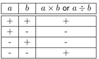
Table 2.1 shows how to calculate the sign of the answer when you multiply two numbers together. The first column shows the sign of the first number, the second column gives the sign of the second number, and the third column shows what sign the answer will be. So multiplying or

a b a_×bora_÷b

+ + +

+ -

-- +

-- - +

Table 2.1: Table of signs for multiplying or dividing two numbers.

dividing a negative number by a positive number always gives you a negative number, whereas multiplying or dividing numbers which have the same sign always gives a positive number. For example,2×3 = 6and−2× −3 = 6, but−2×3 =−6and2× −3 =−6.

Adding numbers works slightly differently, have a look at Table 2.2. The first column shows the sign of the first number, the second column gives the sign of the second number, and the third column shows what sign the answer will be.

a b a+b

+ + +

+ - ?

- + ?

- -

-Table 2.2: -Table of signs for adding two numbers.

(32)

If you add two positive numbers you will always get a positive number, but if you add two negative numbers you will always get a negative number. If the numbers have different sign, then the sign of the answer depends on which one is bigger.

2.8.3 Living Without the Number Line

The number line in Figure 2.1 is a good way to visualise what negative numbers are, but it can get very inefficient to use it every time you want to add or subtract negative numbers. To keep things simple, we will write down three tips that you can use to make working with negative numbers a little bit easier. These tips will let you work out what the answer is when you add or subtract numbers which may be negative and will also help you keep your work tidy and easier to understand.

Negative Numbers Tip 1

If you are given an equation like₋a+b, then it is easier to move the numbers around so that the equation looks easier. For this case, we have seen that adding a negative number to a positive number is the same as subtracting the number from the positive number. So,

−a+b = b₋a (2.17)

−5 + 10 = 10₋5 = 5

This makes equations easier to understand. For example, a question like “What is₋7 + 11?” looks a lot more complicated than “What is11₋7?”, even though they are exactly the same question.

When you have two negative numbers like−3−7, you can calculate the answer by simply adding together the numbers as if they were positive and then putting a negative sign in front.

−c−d = −(c+d) (2.18)

−7₋2 = ₋(7 + 2) =₋9

In Table 2.2 we saw that the sign of two numbers added together depends on which one is bigger. This tip tells us that all we need to do is take the smaller number away from the larger one, and remember to put a negative sign before the answer if the bigger number was subtracted to begin with. In this equation,F is bigger thane.

e₋F = ₋(F₋e) (2.19)

2−11 = −(11−2) =−9

You can even combine these tips together, so for example you can use Tip 1 on₋10 + 3to get

3₋10, and then use Tip 3 to get ₋(10₋3) =₋7.

Exercise: Negative Numbers 1. Calculate:

(a)(₋5)₋(₋3) (b) (₋4) + 2 (c)(₋10)_÷(₋2)

(d)11₋(₋9) (e)₋16₋(6) (f)₋9_÷3_×2

(g)(₋1)_×24_÷8_×(₋3) (h) (₋2) + (₋7) (i)1₋12

(j)3₋64 + 1 (k)₋5₋5₋5 (l)₋6 + 25

(33)

2. Say whether the sign of the answer is + or -(a)₋5 + 6 (b) ₋5 + 1 (c) ₋5_{÷ −}5

(d)₋5_÷5 (e)5_{÷ −}5 (f) 5_÷5

(g)₋5_{× −}5 (h) ₋5_×5 (i) 5_{× −}5

(j)5_×5

2.9 Rearranging Equations

Now that we have described the basic rules of negative and positive numbers and what to do when you add, subtract, multiply and divide them, we are ready to tackle some real mathematics problems!

Earlier in this chapter, we wrote a general equation for calculating how much change (x) we can expect if we know how much an item costs (y) and how much we have given the cashier (z). The equation is:

x+y=z (2.20)

So, if the price is R10 and you gave the cashier R15, then write R15 instead ofzand R10 instead ofy.

x+ 10 = 15 (2.21)

Now, that we have written this equation down, how exactly do we go about finding what the change is? In mathematical terms, this is known as solving an equation for an unknown (x in this case). We want to re-arrange the terms in the equation, so that onlyxis on the left hand side of the=sign and everything else is on the right.

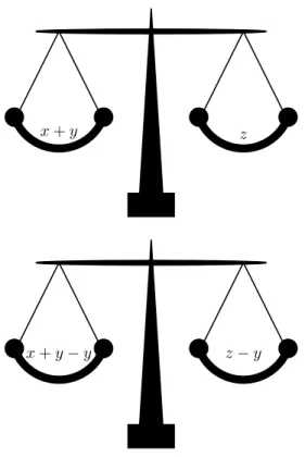
The most important thing to remember is that an equation is like a set of weighing scales. In order to keep the scales balanced, whatever, is done to one side, must be done to the other.

Method: Rearranging Equations

You can add, subtract, multiply or divide both sides of an equation by any number you want, as long as you always do it to both sides.

So for our example we could subtracty from both sides

x+y = z (2.22)

x+y₋y = z₋y

x = z₋y

x = 15−10

= 5

so now we can find the change is the price subtracted from the amount handed over to the cashier. In the example, the change should be R5. In real life we can do this in our head, the human brain is very smart and can do arithmetic without even knowing it.

When you subtract a number from both sides of an equation, it looks just like you moved a positive number from one side and it became a negative on the other, which is exactly what happened. Likewise if you move a multiplied number from one side to the other, it looks like it changed to a divide. This is because you really just divided both sides by that number, and a

(34)

x+y z

x+y−y z−y

divide the other side too.

Figure 2.2: An equation is like a set of weighing scales. In order to keep the scales balanced, you must do the same thing to both sides. So, if you add, subtract, multiply or divide the one side, you must add, subtract, multiply or

divide the other side too.

number divided by itself is just1

a(5 +c) = 3a (2.23)

a(5 +c)_÷a = 3a_÷a a

a×(5 +c) = 3× a a

1_×(5 +c) = 3_×1 5 +c = 3

c = 3−5 =−2

However you must be careful when doing this, as it is easy to make mistakes. The following is the wrong thing to do

5a+c = 3a (2.24)

5 +c ₆=4 ₃_a

÷a

Can you see why it is wrong? It is wrong because we did not divide thecterm byaas well. The correct thing to do is

5a+c = 3a (2.25)

5 +c_÷a = 3

c÷a = 3−5 =−2

(35)

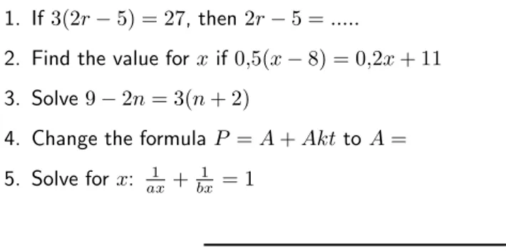
1. If3(2r₋5) = 27, then2r₋5 =...

2. Find the value forxif0,5(x₋8) = 0,2x+ 11

3. Solve9₋2n= 3(n+ 2)

4. Change the formulaP =A+AkttoA=

5. Solve forx: _ax1 +_bx1 = 1

2.10 Fractions and Decimal Numbers

A fraction is one number divided by another number. There are several ways to write a number divided by another one, such asa_÷b,a/band a

b. The first way of writing a fraction is very hard

to work with, so we will use only the other two. We call the number on the top, thenumerator and the number on the bottom thedenominator. For example,

1 5

numerator = 1

denominator = 5 (2.26)

Extension: Definition - Fraction The wordfractionmeanspart of a whole.

Thereciprocal of a fraction is the fraction turned upside down, in other words the numerator becomes the denominator and the denominator becomes the numerator. So, the reciprocal of 2 3

is 3 2.

A fraction multiplied by its reciprocal is always equal to1and can be written

a b ×

b

a = 1 (2.27)

This is because dividing by a number is the same as multiplying by its reciprocal.

Extension: Definition - Multiplicative Inverse

The reciprocal of a number is also known as the multiplicative inverse.

A decimal number is a number which has an integer part and a fractional part. The integer and the fractional parts are separated by adecimal point, which is written as a comma in South Africa. For example the number314

100 can be written much more cleanly as3,14.

All real numbers can be written as a decimal number. However, some numbers would take a huge amount of paper (and ink) to write out in full! Some decimal numbers will have a number which will repeat itself, such as0,33333. . .where there are an infinite number of 3’s. We can write this decimal value by using a dot above the repeating number, so 0,˙3 = 0,33333. . .. If there are two repeating numbers such as0,121212. . .then you can place dots5 _{on each of the} repeated numbers0,˙1˙2 = 0,121212. . .. These kinds of repeating decimals are called recurring decimals.

Table 2.3 lists some common fractions and their decimal forms.

5_{or a bar, like}₀_,₁₂

(36)

Fraction Decimal Form

1

20 0,05 1

16 0,0625

1

10 0,1 1

8 0,125

1

6 0,16 ˙6 1

5 0,2 1

2 0,5 3

4 0,75

Table 2.3: Some common fractions and their equivalent decimal forms.

2.11 Scientific Notation

In science one often needs to work with very large or very small numbers. These can be written more easily in scientific notation, which has the general form

a_×10m (2.28)

whereais a decimal number between 0 and 10 that is rounded off to a few decimal places. The

mis an integer and if it is positive it represents how many zeros should appear to the right of

a. Ifmis negative then it represents how many times the decimal place in ashould be moved to the left. For example3,2_×103 _{represents 32000 and}₃_,₂

×10−3_represents₀_,₀₀₃₂_.

If a number must be converted into scientific notation, we need to work out how many times the number must be multiplied or divided by 10 to make it into a number between 1 and 10 (i.e. we need to work out the value of the exponentm) and what this number is (the value of

a). We do this by counting the number of decimal places the decimal point must move. For example, write the speed of light which is 299 792 458ms−1 _{in scientific notation, to two}

decimal places. First, determine where the decimal point must go for two decimal places (to finda) and then count how many places there are after the decimal point to determinem. In this example, the decimal point must go after the first 2, but since the number after the 9 is a 7,a= 3,00.

So the number is 3,00_×10m_{, where}_m _{= 8}_{, because there are 8 digits left after the decimal}

point. So the speed of light in scientific notation, to two decimal places is3,00_×108_ms−1_.

As another example, the size of the HI virus is around120_×10−9 _{m. This is equal to} ₁₂₀

×

0,000000001m which is 0,00000012 m.

2.12 Real Numbers

Now that we have learnt about the basics of mathematics, we can look at what real numbers are in a little more detail. The following are examples of real numbers and it is seen that each number is written in a different way.

√

3, 1,2557878, 56

34, 10, 2,1, −5, −6,35, − 1

90 (2.29)

(37)

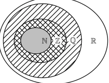
R Q Z N

Figure 2.3: Set diagram of all the real numbersR, the rational numbers Q, the integersZand the natural numbersN. The irrational numbers are the numbers not inside the set of rational numbers. All of the integers are also rational numbers, but not all rational numbers are integers.

Extension: Non-Real Numbers

All numbers that are not real numbers haveimaginary components. We will not see imaginary numbers in this book but you will see that they come from√−1. Since we won’t be looking at numbers which are not real, if you see a number you can be sure it is a real one.

2.12.1 Natural Numbers

The first type of numbers that are learnt about are the numbers that were used for counting. These numbers are callednatural numbers and are the simplest numbers in mathematics.

0,1,2,3,4. . . (2.30)

Mathematicians use the symbolNto mean theset of all natural numbers. The natural numbers are asubset of the real numbers since every natural number is also a real number.

2.12.2 Integers

The integers are all of the natural numbers and their negatives

. . .−4,−3,−2,−1,0,1,2,3,4. . . (2.31) Mathematicians use the symbolZto meanthe set of all integers. The integers are a subset of the real numbers, since every integer is a real number.

2.12.3 Rational Numbers

The natural numbers and the integers are only able to describe quantities that are whole or complete. For example you can have 4 apples, but what happens when you divide one apple into 4 equal pieces and share it among your friends? Then it is not a whole apple anymore and a different type of number is needed to describe the apples. This type of number is known as a rational number.

A rational number is any number which can be written as:

a

b (2.32)

whereaandb are integers andb₆= 0.

The following are examples of rational numbers:

20 9 ,

−1 2 ,

20 10,

3

15 (2.33)

(38)

Extension: Notation Tip

Rational numbers are any number that can be expressed in the forma

b;a, b∈Z;b6= 0

which means “the set of numbers a_b whenaandbare integers”.

Mathematicians use the symbolQto meanthe set of all rational numbers. The set of rational numbers contains all numbers which can be written as terminating or repeating decimals.

Extension: Rational Numbers

All integers are rational numbers with denominator1.

You can add and multiply rational numbers and still get a rational number at the end, which is very useful. If we have 4 integers,a, b, candd, then the rules for adding and multiplying rational numbers are

a b +

c

d =

ad+bc

bd (2.34)

a b ×

c

d =

ac

bd (2.35)

Extension: Notation Tip

The statement ”4 integersa, b, candd” can be written formally as_{a, b, c, d_{} ∈}Z because the_∈symbol meansinand we say thata, b, canddareinthe set of integers.

Two rational numbers (a_b and _dc) represent the same number if ad = bc. It is always best to simplify any rational number so that the denominator is as small as possible. This can be achieved by dividing both the numerator and the denominator by the same integer. For example, the rational number1000/10000can be divided by 1000 on the top and the bottom, which gives

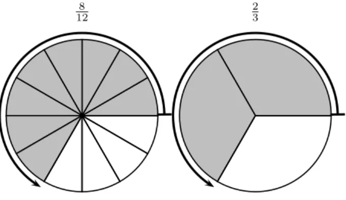
1/10. 2₃ of a pizza is the same as ₁₂8 (Figure 2.4).

8 12

2 3

Figure 2.4: ₁₂8 of the pizza is the same as 2₃ of the pizza.

You can also add rational numbers together by finding alowest common denominator and then adding the numerators. Finding a lowest common denominator means finding the lowest number that both denominators are afactor6_{of. A factor of a number is an integer which evenly divides} that number without leaving a remainder. The following numbers all have a factor of 3

3,6,9,12,15,18,21,24. . .

and the following all have factors of 4

4,8,12,16,20,24,28. . .

(39)

The common denominators between 3 and 4 are all the numbers that appear in both of these lists, like 12 and 24. The lowest common denominator of 3 and 4 is the number that has both 3 and 4 as factors, which is 12.

For example, if we wish to add 3₄ + 2₃, we first need to write both fractions so that their denominators are the same by finding the lowest common denominator, which we know is 12. We can do this by multiplying 3₄ by 3₃ and 2₃ by 4₄. 3₃ and 4₄ are really just complicated ways of writing1. Multiplying a number by1doesn’t change the number.

3 4+ 2 3 = 3 4× 3 3+ 2 3 × 4 4 (2.36)

= 3×3 4_×3 +

2×4 3_×4

= 9

12+ 8 12

= 9 + 8 12

= 17 12

Dividing by a rational number is the same as multiplying by its reciprocal, as long as neither the numerator nor the denominator is zero:

a b ÷ c d = a b. d c = ad bc (2.37)

A rational number may be aproper orimproper fraction.

Proper fractions have a numerator that is smaller than the denominator. For example,

−1 2 , 3 15, −5 −20

are proper fractions.

Improper fractions have a numerator that is larger than the denominator. For example,

−10 2 , 13 15, −53 −20

are improper fractions. Improper fractions can always be written as the sum of an integer and a proper fraction.

Converting Rationals into Decimal Numbers Converting rationals into decimal numbers is very easy.

If you use a calculator, you can simply divide the numerator by the denominator. If you do not have a calculator, then you unfortunately have to use long division.

Since long division, was first taught in primary school, it will not be discussed here. If you have trouble with long division, then please ask your friends or your teacher to explain it to you.

2.12.4 Irrational Numbers

An irrational number is any real number that is not a rational number. When expressed as decimals these numbers can never be fully written out as they have an infinite number of decimal places which never fall into a repeating pattern, for example √2 = 1,41421356. . .,

π= 3,14159265. . .. πis a Greek letter and is pronounced “pie”.

Exercise: Real Numbers

(40)

1. Identify the number type (rational, irrational, real, integer) of each of the following numbers:

(a) c

d if cis an integer and if dis irrational.

(b) 3 2

(c) -25 (d) 1,525 (e) √10

2. Is the following pair of numbers real and rational or real and irrational? Explain._√

4;1 8

2.13 Mathematical Symbols

The following is a table of the meanings of some mathematical signs and symbols that you should have come across in earlier grades.

Sign or Symbol Meaning

> greater than

< less than

≥ greater than or equal to

≤ less than or equal to

So if we writex > 5, we say thatxis greater than 5 and if we writex≥y, we mean thatx

can be greater than or equal toy. Similarly, < means ‘is less than’ and≤means ‘is less than or equal to’. Instead of saying thatxis between6and10, we often write6<10. This directly means ‘six is less thanxwhich in turn is less than ten’.

Exercise: Mathematical Symbols 1. Write the following in symbols:

(a) xis greater than 1 (b) y is less than or equal toz

(c) ais greater than or equal to 21

(d) pis greater than or equal to 21 andpis less than or equal to 25

2.14 Infinity

Infinity (symbol∞) is usually thought of as something like “the largest possible number” or “the furthest possible distance”. In mathematics, infinity is often treated as if it were a number, but it is clearly a very different type of “number” than the integers or reals.

(41)

2.15 End of Chapter Exercises

1. Calculate (a) 18₋6_×2

(b) 10 + 3(2 + 6)

(c) 50₋10(4₋2) + 6

(d) 2_×9₋3(6₋1) + 1

(e) 8 + 24÷4×2

(f) 30−3×4 + 2

(g) 36÷4(5−2) + 6

(h) 20₋4_×2 + 3

(i) 4 + 6(8 + 2)₋3

(j) 100₋10(2 + 3) + 4

2. Ifp=q+ 4r, thenr=...

3. Solve x−2

3 =x−3

(42)

(43)

Chapter 3

Rational Numbers - Grade 10

3.1 Introduction

As described in Chapter 2, a number is a way of representing quantity. The numbers that will be used in high school are all real numbers, but there are many different ways of writing any single real number.

This chapter describesrational numbers.

3.2 The Big Picture of Numbers

Real Numbers

Irrationals Rationals

Integers Whole

Natural All numbers inside

the grey oval are ra-tional numbers.

3.3 Definition

The following numbers are all rational numbers.

10 1 ,

21 7 ,

−1

−3, 10 20,

−3

6 (3.1)

You can see that all the denominators and all the numerators are integers1_.

Definition: Rational Number

A rational number is any number which can be written as:

a

b (3.2)

where aandb are integers andb6= 0.

1_{Integers are the counting numbers (1, 2, 3, ...), their opposites (-1, -2, -3, ...), and 0.}

(44)

Important: Only fractions which have a numerator and a denominator that are integers are rational numbers.

This means that all integers are rational numbers, because they can be written with a denominator of 1.

Therefore, while _√

2 7 ,

−1,33

−3 ,

π

20,

−3

6,39 (3.3)

are not examples of rational numbers, because in each case, either the numerator or the denominator is not an integer.

Exercise: Rational Numbers

1. Ifais an integer,bis an integer andcis not an integer, which of the following are rational numbers:

(a) 5

6 (b)

a

3 (c)

b

2 (d) 1

c

2. If a₁ is a rational number, which of the following are valid values fora? (a)1 (b)−10 (c)√2 (d)2,1

3.4 Forms of Rational Numbers

All integers and fractions with integer numerators and denominators are rational numbers. There are two more forms of rational numbers.

Activity :: Investigation : Decimal Numbers

You can write the rational number 1₂ as the decimal number 0,5. Write the following numbers as decimals:

1. 1₄ 2. ₁₀1 3. 2

5

4. ₁₀₀1 5. 2₃

Do the numbers after the decimal comma end or do they continue? If they continue, is there a repeating pattern to the numbers?

You can write a rational number as a decimal number. Therefore, you should be able to write a decimal number as a rational number. Two types of decimal numbers can be written as rational numbers:

(45)

2. decimal numbers that have a repeating pattern of numbers, for example the fraction 1 3

can be written as0,333333.

For example, the rational number 5₆ can be written in decimal notation as0,83333, and similarly, the decimal number 0,25 can be written as a rational number as 1₄.

Important: Notation for Repeating Decimals

You can use a bar over the repeated numbers to indicate that the decimal is a repeating decimal.

3.5 Converting Terminating Decimals into Rational

Num-bers

A decimal number has an integer part and a fractional part. For example,10,589has an integer part of10and a fractional part of0,589because10 + 0,589 = 10,589. The fractional part can be written as a rational number, i.e. with a numerator and a denominator that are integers. Each digit after the decimal point is a fraction with denominator in increasing powers of ten. For example:

• 1 10 is 0,1

• 1

100 is 0,01

This means that:

2,103 = 2 + 1 10+

0 100+

3 1000

= 2 103 1000

= 2103 1000

Exercise: Fractions

1. Write the following as fractions:

(a)0,1 (b)0,12 (c)0,58 (d)0,2589

3.6 Converting Repeating Decimals into Rational Numbers

When the decimal is a repeating decimal, a bit more work is needed to write the fractional part of the decimal number as a fraction. We will explain by means of an example.

If we wish to write0,3 in the form a_b (where a and b are integers) then we would proceed as follows

x = 0,33333. . . (3.4)

10x = 3,33333. . . multiply by 10 on both sides (3.5)

9x = 3 subtracting (3.4) from (3.5)

x = 3

9 = 1 3

(46)

And another example would be to write5,432as a rational fraction

x = 5,432432432. . . (3.6)

1000x = 5432,432432432. . . multiply by 1000 on both sides (3.7)

999x = 5427 subtracting (3.6) from (3.7)

x = 5427

999 = 201

37

For the first example, the decimal number was multiplied by 10 and for the second example, the decimal number was multiplied by 1000. This is because for the first example there was only one number (i.e. 3) that recurred, while for the second example there were three numbers (i.e. 432) that recurred.

In general, if you have one number recurring, then multiply by 10, if you have two numbers recurring, then multiply by 100, if you have three numbers recurring, then multiply by 1000. Can you spot the pattern yet?

The number of zeros after the 1 is the same as the number of recurring numbers.

But not all decimal numbers can be written as rational numbers, because some decimal numbers like√2 = 1,4142135...is an irrational number and cannot be written with an integer numerator and an integer denominator. However, when possible, you should always use rational numbers or fractions instead of decimals.

Exercise: Repeated Decimal Notation

1. Write the following using the repeated decimal notation: (a) 0,11111111. . .

(b) 0,1212121212. . .

(c) 0,123123123123. . .

(d) 0,11414541454145. . .

2. Write the following in decimal form, using the repeated decimal notation: (a) 2₃

(b) 1₁₁3

(c) 45 6

(d) 21 9. . .

3. Write the following decimals in fractional form: (a) 0,6333. . .

(b) 5,313131

(c) 11,570571. . .

(d) 0,999999. . .

3.7 Summary

The following are rational numbers:

• Fractions with both denominator and numerator as integers.

• Integers.

• Decimal numbers that end.

(47)

3.8 End of Chapter Exercises

1. Ifais an integer,bis an integer andcis not an integer, which of the following are rational numbers:

(a) 5₆ (b) a₃ (c) b₂ (d) 1_c

2. Write each decimal as a simple fraction: (a) 0,5

(b) 0,12

(c) 0,6

(d) 1,59

(e) 12,277

3. Show that the decimal3,2 ˙1˙8is a rational number.

4. Showing all working, express0,7 ˙8as a fraction a_b wherea, b∈Z.

(48)

(49)

Chapter 4

Exponentials - Grade 10

4.1 Introduction

In this chapter, you will learn about the short-cuts to writing2_×2_×2_×2. This is known as writing a number inexponential notation.

4.2 Definition

Exponential notation is a short way of writing the same number multiplied by itself many times. For example, instead of5_×5_×5, we write53_{to show that the number 5 is multiplied by itself}

3 times and we say “5 to the power of 3”. Likewise52_is₅

×5and35_is₃

×3_×3_×3_×3. We will now have a closer look at writing numbers using exponential notation.

Definition: Exponential Notation

Exponential notation means a number written like

an

whennis an integer andacan be any real number. ais called thebase andnis called the exponent.

Thenth power ofais defined as:

an= 1_×a_×a_×. . ._×a (n times) (4.1)

withamultiplied by itselfntimes.

We can also define what it means if we have a negative index,−n. Then,

a−n= 1÷a÷a÷. . .÷a (ntimes) (4.2)

Important: Exponentials

If n is an even integer, then an _{will always be positive for any non-zero real number} _a_{. For}

example, although₋2 is negative,(₋2)2 _{= 1}

× −2_{× −}2 = 4 is positive and so is(₋2)−2 ₌

1÷ −2÷ −2 = 1₄.

FHSST Mathematics for Grade 10 - 12 - Free Computer, Programming, Mathematics, Technical Books, Lecture Notes and Tutorials

FHSST Authors

The Free High School Science Texts:

Textbooks for High School Students

Studying the Sciences

Mathematics

Grades 10 - 12

STOP!!!!

Did you notice the FREEDOMS we’ve granted you?

Our copyright license is

different!

It grants freedoms

rather than just imposing restrictions like all those other

textbooks you probably own or use.

•

We know people copy textbooks illegally but we would LOVE it if you copied

our’s - go ahead copy to your hearts content,

legally!

•

Publishers revenue is generated by controlling the market, we don’t want any

money, go ahead, distribute our books far and wide - we DARE you!

•

Ever wanted to change your textbook? Of course you have! Go ahead change

ours, make your own version, get your friends together, rip it apart and put

it back together the way you like it. That’s what we really want!

•

Copy, modify, adapt, enhance, share, critique, adore, and contextualise. Do it

all, do it with your colleagues, your friends or alone but get involved! Together

we can overcome the challenges our complex and diverse country presents.

•

So what is the catch? The only thing you can’t do is take this book, make

a few changes and then tell others that they can’t do the same with your

changes. It’s share and share-alike and we know you’ll agree that is only fair.

FHSST Core Team

FHSST Editors

FHSST Contributors

www.fhsst.org

Contents

I

Basics

1

II

Grade 10

5

III

Grade 11

249

V

Exercises

613

Part I

Basics

Chapter 1

Introduction to Book

1.1

The Language of Mathematics

Part II

Grade 10

Chapter 2

Review of Past Work

2.1

Introduction

2.2

What is a number?

2.3

Sets

2.4

Letters and Arithmetic

2.5

Addition and Subtraction

2.6

Multiplication and Division

2.7

Brackets

2.8

Negative Numbers

2.8.1

What is a negative number?

2.8.2

Working with Negative Numbers