The Early-Time (E1) High-Altitude Electromagnetic Pulse (HEMP) and Its Impact on the U.S. Power Grid

Meta-R-320

The Early-Time (E1) High-Altitude

Electromagnetic Pulse (HEMP) and

Its Impact on the U.S. Power Grid

Edward Savage

James Gilbert

William Radasky

Metatech Corporation

358 S. Fairview Ave., Suite E

Goleta, CA 93117

January 2010

Prepared for

Oak Ridge National Laboratory

Attn: Dr. Ben McConnell

1 Bethel Valley Road

P.O. Box 2008

Oak Ridge, Tennessee 37831

Subcontract 6400009137

FOREWORD

This report describes the threat of the early-time (E1) high-altitude electromagnetic pulse (HEMP) produced by nuclear detonations above an altitude of ~30 km. The report describes the mechanisms that create the E1 HEMP, the evidence for concern about this threat, and how it can impact the U.S. power grid. As the late-time (E3) part of the HEMP is considerably different in its frequency content and how it affects the power grid, this aspect will be discussed in another report.

This report is organized to provide an introduction to the report in Section 1, followed by an overview of E1 HEMP in Section 2. Section 3 then provides a brief history of E1 HEMP experience. Section 4 discusses in some detail how the E1 HEMP is generated for those who have more interest in the physics of the problem. Section 5 presents details concerning the coupling of these fields to extended lines, while Section 6 describes vulnerabilities of electronics to this threat. In Section 7 there is a detailed discussion of the main concerns of E1 HEMP on the U.S. power grid, and this section is crucial to set the stage to describe and recommend protection approaches and methods in the future. Section 8 follows with a brief discussion of potential impacts of large-scale power outages on society. Section 9 provides a bibliography highlighting some of the most important papers dealing with the E1 threat, standards to deal with the impacts of the threat, and recent publications produced for the EMP Commission and other groups related to the vulnerability of different aspects of the U.S. power system to electromagnetic threats. Finally, an appendix discusses some common E1 HEMP myths.

Table of Contents

Section Page 1 Introduction... 1-1

2 An Overview of E1 HEMP ...2-1 2.1 Historical Prospective ...2-1 2.2 E1 HEMP Environment ...2-2 2.3 Some Similar Effects...2-6 2.4 Other Types of EMP ...2-7 2.5 Parameters That Control E1 HEMP ...2-11 2.6 HOB Variation ...2-13 2.7 Exposed Region...2-14 2.8 E1 HEMP Geometry Features...2-16 2.9 Incident and Total E1 HEMP Environments...2-19 2.10 Generic E1 HEMP Environment...2-21 2.11 Energy Conservation Check...2-25 2.12 E1 HEMP: Instantaneous and Simultaneous...2-27 2.13 Observer Location Variation (Smile Diagram) and Observed Function...2-28 2.14 E1 HEMP Effects on Systems...2-35 2.15 E1 HEMP Coupling ...2-37 2.16 E1 HEMP Penetration and Protection...2-40 2.17 E1 HEMP Specifications...2-43 2.18 Effects on Power Grid and Society ...2-44 3 A Brief History of E1 HEMP Experiences ...3-1 4 E1 HEMP Generation and Environments ...4-1 4.1 E1 HEMP Generation...4-1 4.2 Conductivity- Air Chemistry...4-6 4.3 E1 HEMP Modeling...4-13 4.4 E1 HEMP Decomposition...4-22 4.5 Field Directions, East-West Symmetry, and Special Points ...4-28 4.6 Some Simplifications ...4-39 5 E1 HEMP Line Coupling...5-1 6 E1 HEMP Vulnerabilities ...6-1 7 Electric Power System E1 HEMP Impacts ...7-1 7.1 E1 HEMP Coupling to Randomly Oriented Lines...7-1 7.2 Susceptibility of Power System Equipment ...7-7 7.3 High Voltage Substation Controls and Communications ...7-19 7.4 Power Generation Facilities ...7-25 7.5 Power Control Centers ...7-25 7.6 Distribution Line Insulators ...7-25 7.6.1 Insulator Testing at MSU...7-27 7.6.2 Insulator Testing in Russia...7-30 7.7 Distribution Transformers ...7-34 8 Impacts on Society of E1 HEMP Power System Failures ...8-1

Section Page 9 Bibliography of E1 HEMP References ...9-1

9.1 General E1 HEMP References...9-1 9.2 IEC HEMP References...9-3 9.3 EMP Commission and Related References...9-7

Appendix Page E1 HEMP Myths... A-1

List of Figures

Figure Page 2-1 The various parts of a generic HEMP signal...2-2

2-2 General basis of the E1 HEMP generation process...2-3 2-3 A sample E1 HEMP “smile” diagram...2-4 2-4 Some similar EM situations. ...2-6 2-5 Approximate EM spectrums for various EM disturbances. ...2-7 2-6 Sample E1 HEMP HOB variation...2-13 2-7 Radius of the E1 HEMP exposed region on the Earth versus the burst height. ..2-14 2-8 E1 HEMP exposed region area versus burst height. ...2-15 2-9 Samples of E1 HEMP exposed regions for several heights. ...2-15 2-10 Explanation of smile diagram variation along the center north/south line...2-16 2-11 Positions of two special E1 HEMP points versus burst height. ...2-18 2-12 Decomposing an incident E1 HEMP into two E field terms for reflection...2-20 2-13 E1 HEMP Earth reflection. ...2-20 2-14 Sample E field signals for E1 HEMP and FM radio. ...2-24 2-15 Spectrum of the idealized E1 HEMP E field signal. ...2-24 2-16 Geometry used in an energy calculation for E1 HEMP. ...2-26 2-17 Sample E1 HEMP peak contours. ...2-30 2-18 Sample E horizontal component contours...2-30 2-19 Sample E north/south horizontal component contours...2-31 2-20 Sample E east/west horizontal component contours. ...2-31 2-21 Horizontal E field direction for E1 HEMP sample. ...2-32 2-22 Sample E vertical component contours. ...2-32 2-23 Peak horizontal E1 HEMP contours, including ground reflection...2-33 2-24 Peak vertical E1 HEMP contours, including ground reflection. ...2-33 2-25 Sample E1 HEMP total energy contours...2-34 2-26 Contours of energy in the 10 to 100 MHz band. ...2-34 2-27 Flash and sparks from pulse damage testing...2-36 2-28 Capacitive (electric) coupling to a short cable. ... 2-38 2-29 Inductance (magnetic) coupling to a short cable...2-38 2-30 Sample contour plot of the peak current on a north/south line. ...2-39 2-31 Sample contour plot of the peak current on an east/west line. ...2-39 2-32 Sample contour plot of the peak current on a vertical wire...2-40 2-33 Electric leakage through an aperture...2-41 2-34 Magnetic leakage through an aperture. ...2-41 2-35 External cabling with poor termination at the subsystem. ...2-43 3-1 Comparison of measured and calculated E1 HEMP signal...3-3 3-2 Geometry of the Starfish test...3-5 3-3 Soviet HEMP test experience...3-6 4-1 Compton scattering...4-1 4-2 Detailed representation of the E1 HEMP generation process. ...4-2 4-3 Details of the E1 HEMP generation in the source region. ...4-4

Figure ... Page 4-4 Representation of the generation of E1 HEMP. ...4-5 4-5 Laboratory E1 HEMP generation experiment...4-5 4-6 Air conductivity calculated with equilibrium secondary electron model...4-12 4-7 Air conductivity calculated with early-time hot secondary electron model...4-13 4-8 Overview of E1 HEMP generation theory terms. ...4-15 4-9 Overview of the source and conductivity terms, including air chemistry...4-15 4-10 Terms and vector directions for the E1 HEMP equation derivation. ...4-17 4-11 Idealization of the E1 HEMP as two terms. ...4-27 4-12 Extending one E1 HEMP calculation to other cases...4-28 4-13 Simple E1 HEMP case. ...4-31 4-14 Including the quadrupole term in the simple case...4-31 4-15 Effect of tilted (non-vertical) geomagnetic field for the simple case...4-32 4-16 Symmetry for the E1 HEMP east-west component...4-34 4-17 Symmetry for the E1 HEMP north-south component...4-34 4-18 Symmetry for the E1 HEMP vertical component. ...4-35 4-19 Close up of the center of the vertical field result in Figure 4-18...4-35 4-20 Field direction variation along a north-south central line. ...4-36 4-21 Loss of east-west symmetry for E1 HEMP components...4-37 4-22 The two orthogonal systems for E1 HEMP. ...4-37 4-23 Single ray approximation. ...4-39 4-24 Exposed region approximation...4-40 5-1 Side view of the line coupling...5-3 5-2 Top view of the line coupling...5-3 5-3 Line coupling geometry...5-4 6-1 A part (a resistor) exploding under pulse testing. ...6-1 6-2 Capacitor damage from pulse testing. ...6-2 6-3 The result of pulse testing – IC damage. ...6-2 6-4 Sample Wunsch-Bell power damage levels versus signal pulse width...6-6 6-5 Sample Wunsch-Bell energy damage level...6-6 6-6 Arcing in a PLC (programmable logic controller). ...6-9 6-7 Arcing at the port to a system...6-10 6-8 Signs of arcing between solder pads on a circuit card. ...6-10 6-9 Arcing occurring near the port entry point, or deeper within the system...6-11 6-10 Arcing used for protection...6-11 7-1 Voltage distribution for a 100-meter long horizontal power line...7-3 7-2 Voltage distribution for a 300-meter long horizontal power line...7-4 7-3 Voltage distribution for a 1000-meter long horizontal power line...7-4 7-4 Voltage distribution for a 10-meter long horizontal control/sensor line. ...7-5 7-5 Voltage distribution for a 30-meter long horizontal control/sensor line. ...7-6 7-6 Voltage distribution for a 100-meter long horizontal control/sensor line. ...7-6 7-7 Voltage distribution for a 4-meter long vertical control/sensor line. ...7-7 7-8 GE-PJC electromechanical overcurrent relay. ...7-10 7-9 GE-GCX electromechanical distance relay...7-11

Figure ... Page 7-10 Modern relay unit. ...7-11 7-11 Inside the SEL-311L electronic relay unit. ...7-12 7-12 Modern SCADA unit...7-12 7-13 Sample pulse test shot result. ...7-14 7-14 The Fisher ROC809 Remote Operations Controller. ...7-16 7-15 The Allen-Bradley MicroLogix 1000 PLC. ...7-17 7-16 Exposure area for E1 HEMP burst at 170 km over Ohio...7-20 7-17 EHV substations in the exposed region shown in Figure 7-16. ...7-20 7-18 Exposure of cable conduits on transformers. ...7-21 7-19 Long runs of “buried” cables in low conductivity gravel. ...7-22 7-20 Second view of cable trenway...7-22 7-21 Control cables in trenway...7-23 7-22 Grounding of control cable shields and j-boxes in control building. ...7-23 7-23 Distribution of control cables within building to cabinets. ...7-24 7-24 A typical above ground 15 kV distribution geometry in the U.S...7-26 7-25 Insulators tested...7-28 7-26 Suspension glass insulator for 10 kV power line. ...7-30 7-27 Snapshots from an insulator test shot, with damage due to power follow. ...7-33 8-1 An example of the failure of an infrastructure system due to EM assault. ...8-2

List of Tables

Table Page 2-1 Typical distribution of energy from a high altitude nuclear explosion. ...2-5

2-2 List of some types of EMP, and other related effects. ...2-9 2-3 List of E1 HEMP input parameters. ...2-11 2-4 Characteristics of the IEC E1 HEMP waveform...2-23 2-5 List of the sample “smile” diagrams. ...2-28 3-1 Early historic EMP events...3-2 4-1 Summary of E1 HEMP generation modeling...4-16 4-2 Vector directions for turned quantities...4-23 4-3 Vector simplifications for the transverse part of the second turning. ...4-25 4-4 Explanation of the two E1 HEMP terms. ...4-26 4-5 The type of east-west symmetry for E1 HEMP components. ...4-37 7-1 List of results for E1 HEMP excitation of lines. ...7-2 7-2 Some previous studies of the response of the power grid to E1 HEMP. ...7-8 7-3 Fast pulse results for relay and SCADA equipment...7-13 7-4 Slow pulse test results for the SEL units...7-14 7-5 Fast pulse results for the Fisher ROC809 unit. ...7-17 7-6 Fast pulse results for the Allen-Bradley MicroLogix 1000 PLC. ...7-18 7-7 Slow pulse results for the Allen-Bradley MicroLogix 1000 PLC...7-18 7-8 Fast pulse results for a typical PC and network switch...7-19 7-9 Summary of the distribution systems for the U.S. power grid...7-26 7-10 Insulator lightning results...7-29 7-11 Insulator fast pulse results. ...7-29 7-12 Effect of pulse type for insulator CFO voltage. ...7-30 7-13 Peak levels of voltage for multiple tests (power off). ...7-31 7-14 Characteristics of insulator number 1 after repeated flashovers (power off). ...7-31 7-15 Peak voltage of flashover for insulators under operational voltage. ...7-32 7-16 Characteristics of insulator number 1 after repeated flashovers (power on)...7-32 7-17 7.2 kV/25 kVA transformer failure testing for fast pulses. ...7-34

Section 1 Introduction

This report discusses the threat and impacts of the early-time (E1) HEMP. This is the earliest part of HEMP (high altitude electromagnetic pulse, generated by an exoatmospheric nuclear burst), encompassing the part of the HEMP that runs out to about a microsecond. It has the highest amplitude in the HEMP waveform, and typically rises to that peak fast, often in a few nanoseconds. It is driven by the burst’s gammas – very high energy photons, which are produced by nuclear reactions within the nuclear burst. This discussion does not assume that the reader already has any EMP experience, so it starts at a very tutorial level. It also continues into more advance discussions, and some physics (engineering, etc.) background might be needed to fully appreciate all the details. Including all details, even simple ones, was done because, especially with the Internet, there is much erroneous EMP information available. Much of the best E1 HEMP material is not readily available, and much of what is easily available has inaccuracies. This is especially true for some of the E1 HEMP information on the Internet. For example, burst “yield” is often considered as the measure of a nuclear device, and correctly so for the blast and shock produced by a surface burst. For E1 HEMP the burst yield has much less significance. Maximum E1 HEMP levels on the ground do not correlate well with device yield.

E1 HEMP work has often been done within the classified environment. Two important reasons for this security are:

1.HEMP generation is intimately connected to significant design details of a nuclear weapon.

2.The work might directly, or indirectly, involve the vulnerability levels of U.S. military systems, and we do not want our enemies to know the HEMP levels to which our security forces are hardened.

E1 HEMP development is reflected in numerous government supported technical reports, and many are classified. However there is also much material in open literature, which is applied in this report.

The initial part of the report deals with E1 HEMP in general, and not exclusively with the effects on the electric power system. Toward the end of the report there are sections specifically dealing with the electric power system. Section 2 is an overview of E1 HEMP - an introduction to many aspects of it. Many of these subjects are then covered in more detail later. Section 3 is a very brief history of E1 HEMP work. Section 4 is a detailed look at the generation of E1 HEMP and the modeling of the process. This deals with the production of the electromagnetic (EM) field that propagates down towards the Earth’s surface. Section 5 is about these EM fields “coupling” to conductors – generating voltages and currents. By far, it is these electrical signals that are the main concern for E1 HEMP effects. Section 6 discusses the adverse effects of E1 HEMP – usually from the voltages and currents either temporarily disrupting, or permanently damaging, systems. Section 7 considers possible failures of the electric power system from E1 HEMP. Failures might occur over a very wide area of the U.S., and there undoubtedly

could also be failures to other vital parts of the U.S. infrastructure. Section 8 considers such issues of widespread U.S. infrastructure failures. Section 9 provides a bibliography of E1 HEMP references. Finally, an appendix discusses some common misunderstandings about E1 HEMP.

In the past the Oak Ridge National Laboratory (ORNL) has looked at HEMP effects on the U.S. electric power system. Also, because of special safety concerns, HEMP effects of nuclear power plants were also studied. More recently, the EMP Commission looked into HEMP and the U.S. critical infrastructure, concluding that the electric power system is one of the most significant components that should be worried about. The U.S. military has taken E1 HEMP very seriously for a long time, including hardening and testing efforts. On the civilian side, the problems have not really been addressed. There has been a wide range in the perception of E1 HEMP as a threat. There are skeptics – those that think E1 HEMP does not exist, or that the models are wrong, or the field levels are not as bad as calculated. There are also those who believe we cannot do anything about it – if it happens we will just have to deal with it then. Then there are others that think every electronic device in the country will fail, and we will go back to the Stone Age. There are many such exaggerated scenarios; for example, it is doubtful that more than a very small fraction of vehicles will suddenly stop working – but how long will they be able to run with gasoline supply disruptions from possible electric power grid problems? And much of the open discussions of nuclear burst EM effects deal with E1 HEMP, as it has very large peak fields, and has often been what is meant by the term “HEMP”. However, there are also other parts to HEMP, and E3 HEMP effects could be just as disastrous to the power grid, or even more so in some cases, than E1 HEMP. Many perceptions of E1 HEMP effects, and the feeling that nothing can be done about E1 HEMP vulnerabilities, are also erroneous. Besides accounting for the unlikely chance of a HEMP event, efforts to protect against E1 HEMP effects also tend to have other benefits. There are other intense EM environments, such as lightning, and switching transients in electric substations, for which there is some overlap in protection methods. There is also a growing concern of “IEMI” (intentional electromagnetic interference), in which criminal or terrorist elements purposely generate high electromagnetic levels to cause upset or damage to the operation of electronics in a building or a substation.

It is noted that there are thousands of reports that have been produced in the United States on the topic of E1 HEMP over the past 40 years. It was not possible to reference every possible document of interest. Instead, in Section 9 at the end of this report there is a list of general HEMP references. That section also adds two additional lists of documents. The IEC (International Electrotechnical Commission) has published numerous HEMP related documents, some of which are listed in the first added list. In the second added list there are documents from the congressionally created “Commission to Assess the Threat to the United States from Electromagnetic Pulse (EMP) Attack” (the “EMP Commission”) and also other organizations dealing with HEMP effects on power systems.

Section 2

An Overview of E1 HEMP

In this section we will briefly introduce many aspects about E1 HEMP. Some of it will introduce the subjects that are more thoroughly discussed later, while some will not be discussed further. This material should provide a good basic understanding of E1 HEMP, its effects, and possible protection. There are many subsections, some short and dealing with a very specific issue.

2.1 Historical Prospective

It was anticipated that a nuclear burst would generate electromagnetic signals, and possibly cause problems for electronic equipment. This proved to be true, and a whole range of EM effects from nuclear bursts were discovered and studied over many years. For E1 HEMP, initial hypotheses were inadequate, and actual signal levels proved to be much higher than anticipated. Adequate theories for E1 were not developed until after nuclear testing was moved underground. There has been extensive theoretical and experimental work on E1 HEMP, including from underground nuclear tests.

Besides work for critical military systems, there were also some early efforts for the telephone network – as seen by one of the first E1 HEMP specification waveforms coming from Bell Laboratories. However, in the competitive commercial environment it is understandable that such E1 HEMP hardening did not go forward. Studies were also done by ORNL for various aspects of E1 HEMP effects on the electric power system in the 1980’s. While over the years interest in E1 HEMP tended to lessen in the U.S., recently it has increased worldwide. The recent efforts of the EMP Commission have shown a renewed sense that E1 HEMP should not be completely ignored by the civil infrastructure.

The only direct experience with E1 HEMP was in 1962, when the U.S. and USSR both experimented with a few high altitude nuclear bursts. For the U.S., the bursts were over the wide expanse of the sparsely populated South Pacific. The only real infrastructure was in Hawaii, very far away, and generally consisted of electronic tubes, and power grid relays that were bulky (and hardy) electromechanical devices. There were some upset and damage effects in Hawaii. The Russian experience, which was over land and more pertinent, was over a vast desert region, also with very antiquated infrastructure equipment. They did have damage associated with long lines (communications and power insulators), and also damage to diesel generators and radar systems. Now, more than half a century later, and after all the technical advances in our modern infrastructure (solid state electronics), it is certainty true to say that E1 HEMP is likely to be a bigger problem than it was in 1962.

2.2 E1 HEMP Environment

The term “environment” is generally used to refer to the basic signal generated by a nuclear explosion, irrespective of any system. Electromagnetic fields may be altered by objects, including a system itself. For E1 HEMP, the “E1 environment” usually also means that the ground reflection is ignored – it is just the incident EM signal (this will become clearer below). Including ground reflections greatly complicates the situation, including the need to specify what ground conductivity to use. (Later time HEMP cannot be discussed as an incident wave – those environments can only be given with reference to some assumed ground conductivity.)

E1 HEMP is an electromagnetic signal that is generated by a nuclear burst that explodes high above the Earth – generally said to be “above the atmosphere”. The atmospheric density gradually decreases with altitude, and so often some approximate altitude is given, such as 30 km (18.6 miles). However, E1 HEMP does not really have a firm height-of-burst (HOB) limit, and there is still E1 HEMP generated for lower altitude bursts, although with lower field levels.

E1 HEMP is a fast narrow pulse, typically going up to high electromagnetic field levels not commonly seen from natural events. Figure 2-1 shows a generic waveform for a full HEMP signal – E1 HEMP is the “prompt gamma signal” part that lasts out to about a microsecond. The rest of the signal is much lower, but also much longer in time extent. Very generally, the bigger the system is (including its attached cables), the more that the wider, but lower level, later time HEMP signals could be a concern. The early part of E2 is actually an extension of E1, but at a much lower level, and typically not of much interest compared to E1. The rest of the HEMP signal types involve different mechanisms. These categories also cannot be specified without giving an assumed Earth conductivity.

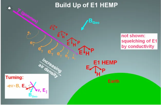
Figure 2-2 shows a general diagram of the E1 HEMP process. A nuclear burst puts out a fast pulse of gamma rays (like x rays, but with higher photon energies – about a few MeV). This thin shell of photons streams outward, including downward toward the Earth and its increasing air density. Once low enough in altitude, the gammas start striking air molecules, knocking electrons off. The Earth’s magnetic field causes the electrons to turn coherently, and this constitutes an electric current, which generates an EM signal, much like the currents on a transmitting antenna. This EM field propagates downward as an EM wave – the E1 signal.

Figure 2-2. General basis of the E1 HEMP generation process. Gammas from the nuclear burst interact with the upper atmosphere – generating Compton electrons, which are turned in the Earth’s geomagnetic field, and produce a transverse current that radiates an EM pulse towards the Earth.

The symbols shown in this figure will be seen in other figures in this report. Specifically, the EM wave has an electric field part “E”, and a corresponding magnetic field part “H”. For an E1 HEMP signal (and EM waves in general), these two terms are perpendicular to each other, and also to the direction of travel (the ray from the burst point to the observer on the Earth). The ray also represents the direction of the “Poynting” vector – giving power (and energy) flow (named after John H. Poynting, but also conveniently “pointing” in the direction of power flow). As shown in the figure, all three vectors are at right angles, and the “right-hand rule” applies: using the right hand, curve fingers in the direction from E to H, and then the thumb points in the direction of P.

The Earth’s magnetic field is traditionally identified by a “B” instead of an “H”. The symbol B is used for the magnetic flux density, and H is used for magnetic field intensity – these two are related by a material’s permeability (which is often about the same as the value for vacuum).

Note that at the ground (Earth’s surface), and up into the atmosphere where humans might be present (at least up to about 50,000 feet – 15 km, 9 miles) there is no weapon radiation – no radioactive particles, no gammas, no x rays, no neutrons, no betas (high energy electrons); just an EM signal, such as in our environment from radio, TV, and as produced by our cell phones.

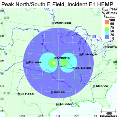
Besides being very strong, the E1 HEMP signal coverage is also very widespread – out to the Earth’s horizon as seen from the burst point. However, for a given weapon and burst location, the E1 HEMP that is seen varies with observer position on the Earth within the exposed region. Figure 2-3 shows a sample variation for the northern hemisphere. This plots the peak of the E field waveform at locations on the Earth (as a fraction of the highest peak seen for all locations). For an obvious reason, contour plots of peak E1 HEMP are often called “smile diagrams” (note the red “lips” with the choice of contour colors used in this example). Here the peak is slightly south of the “Ground Zero” (the point directly below the burst), and there is a low field point (centered on the “null point”) north of Ground Zero. HEMP is governed by the Earth’s magnetic field (geomagnetic field), and so the peak and null points are actually geomagnetically south and north from Ground Zero in the Northern Hemisphere. For E1 HEMP we typically mean geomagnetic, not geographic, directions in our discussions.

Figure 2-3. A sample E1 HEMP “smile” diagram. Such diagrams show contours of peak incident E levels, for a burst height of 75 km in this example. Here contour levels are shown as fractions of the biggest peak level (which is to the south of the burst point for this northern latitude burst). Over the exposed region, the average value is 10.4% of the maximum (12.4% if we use the square root of the average square of the peak instead).

Some of the variation shown in the smile diagram is due to the way the geomagnetic field comes into play in the E1 HEMP generation process. For example, the null point is were the ray from the burst to the observer is parallel to the geomagnetic field lines, while the maximum E1 HEMP point is near where the ray and geomagnetic field are at right angles. There is also an effect from the angle at which the burst-observer ray goes though the Earth’s atmosphere. A ray that enters at a steep angle (the steepest being for GZ – straight down) tends to be higher, faster rising and falling, and possesses more high frequency content, than a ray that enters the atmosphere at a shallower angle (the shallowest being for the outer edges of the exposed region, for rays that are tangent to the Earth’s surface).

E1 HEMP is generated by the gamma rays from a nuclear explosion. Table 2-1 shows a sample set of energy distribution for a high altitude nuclear explosion. (This is for the initial explosion of a high altitude burst. Vastly different values might be found for an air burst, in which energies get transferred to other forms over time – even a very short time.) It can be seen that the gammas are actually a very small fraction of the energy emitted. X rays represent most of the energy from the burst. X rays can play a part in E1 HEMP, but usually only as a limiting effect by producing air conductivity, decreasing the field levels; and then only for the small part of the x-ray output that is high-energy photons, while the vast majority of the x-ray energy is in the part of the spectrum with photons of much lower energy.

Table 2-1. Typical distribution of energy from a high altitude nuclear explosion. The gammas, which generate E1 HEMP, are a small fraction of the total energy.

Energy Fractions of Burst Type Typical

Percentage Source

Typical particle energy X rays (photons) 70 Atomic processes -

electrons 10 keV

Kinetic energy 25 Thermal -

Neutrons 1 Processes in Nucleus 0.01 – 15 MeV Gammas

(photons) 0.1 Nucleus 0.1 - 5 MeV

Energy distribution changes as time evolves, and with differences between surface bursts (in normal air density, such as near the Earth’s surface) and exoatmospheric bursts (in the vacuum of space). A nuclear burst, in a very short time, releases energy as photons (gammas and x rays), neutrons (freed from the nucleus of atoms), betas (energetic electrons), and kinetic energy (atoms and molecules {reactions tend to break apart molecules} with very high velocities). These atoms and molecules are often ionized, having been stripped of many of their electrons. For an air burst, for example, the x rays will be absorbed close to the burst point, and the air will get extremely hot, radiating away light – especially much energy as UV.

2.3 Some Similar Effects

There are some other EM effects that have similarities to E1 HEMP, such as shown in Figure 2-4. Drawing “a” shows a radio transmitter. Current flows up and down the vertical antenna, generating an outward-going EM wave that the radio receiver demodulates into the transmitted music. In drawing “b” there is a lightning cloud-to-ground strike, with its vertical currents, which also sends out EM waves – possibly heard as crackling in the radio receiver (although a direct hit on the radio antenna would most likely damage the receiver, unless there was a very good lightning arrestor attached). In drawing “c” we see that E1 HEMP is also an EM wave – picked up by the radio, it might make a crackle or pop, or silence the radio by causing damage. The last EM example, drawing “d”, shows IEMI – intentional electromagnetic interference. Here someone, for whatever sinister reason, sends out a strong EM signal, trying to disrupt or destroy some electronic system.

Figure 2-4. Some similar EM situations. In drawing “a” the AM radio antenna, using antenna currents produced by the transmitter, radiates an EM signal, which is picked up and demodulated to the music signal sent by the station. In “b” a lightning strike has vertical currents, which generate an EM interference signal (which also can be called a form of EMP, but not HEMP) that is heard as a crackle in the radio receiver. In drawing “c” an E1 HEMP, generated in the upper atmosphere, propagates down to the radio, where it is heard as some interference (such as a crackle or pop), and possibly silence, if the radio is damaged. In “d” a criminal uses a high power RF generator and antenna to disrupt or destroy electronic equipment, such as security devices in a robbery attempt or vital equipment in an extortion scheme.

Figure 2-5 shows an approximate spectral representation of various high-level EM environments, including lightning, E1 HEMP, and wideband and narrowband signals that include IEMI. We see that E1 HEMP dominates in the middle, from about one megahertz to several hundred megahertz. Normal EM noise (“EMI environments”) and radio stations are shown below at the bottom of the chart.

Figure 2-5. Approximate EM spectrums for various EM disturbances. E1 HEMP dominates in the range of about 1 MHz to several hundred MHz. IEMI is represented by the “Wideband” and “Narrowband” signals on the upper frequency (right) side.

2.4 Other Types of EMP

Traditionally “EMP” often refers to E1 HEMP, but it is not the only EM environment produced by a nuclear blast. Table 2-2 lists some other effects that are associated with nuclear blasts or high level EM. The term NEMP (nuclear EMP) is sometimes used to indicate a nuclear burst as the source. HEMP (high-altitude EMP) is also sometimes written with the “a” for “altitude” – HAEMP; or as HABEMP for “high-altitude burst” EMP. HEMP itself has various parts:

E1: early time HEMP; also called prompt gamma HEMP.

E2: intermediate time HEMP, consisting of E2A (scattered gamma HEMP) and E2B (neutron gamma HEMP).

E3: late time HEMP, also called MHD (magnetohydrodynamic) EMP; consisting of the E3A (blast wave) and E3B (heave) MHD.

DEMP (dispersed EMP) is an E1 HEMP signal that propagates back into outer space, either from being above the Earth’s horizon, so missing the ground, or by reflecting off the ground. In going into outer space, it goes through the ionosphere, which distorts the HEMP pulse into a ringing signal.

For bursts within the atmosphere (not “high altitude”) there would also be EM fields generated, but they tend to be small unless the burst is near the Earth’s surface. SREMP is source region EMP, from a burst on or near the Earth’s surface. In this case there would be other nuclear effects that might be of more concern, such as blast damage from the burst itself, but EM effects are of concern for hardened (such as buried) military systems.

SGEMP (system generated EMP) and IEMP (internal EMP) deal with EM effects associated with radiation interaction with a system itself. This can be gammas or x rays producing electrons by colliding with the system molecules. IEMP is a subclass of SGEMP, dealing with radiation penetrating into the interior of a system, where it generates EM fields; while SGEMP itself can also include the generation of fields outside the system, by electrons knocked off the outside. This may be taking place in vacuum, air, or some other gas for the “empty” spaces inside and outside (such as for a satellite or a missile outside the atmosphere).

Nuclear induced lightning (NIL) was observed in high-yield nuclear surface burst tests. This “lightning” was at the edge of the fireball, and so its high current would only be an issue for a hardened system – such as for an antenna connected to a buried system.

For all of the nuclear EM effects we have the disadvantage of a lack of real experience – our current infrastructure has not been exposed to nuclear effects, nor can we fully simulate all of the effects. The closest simulations were for SREMP, SGEMP and IEMP, with small systems in underground tests (when such tests were still being done). Also, there are some high-level gamma and x-ray test machines that, to varying degrees, can simulate nuclear environments for SREMP, SGEMP and IEMP. Some high level EM effects occur naturally, and we do experience them occasionally in our every-day environments. LEMP refers to the EM environment associated with standard lightning. Of course lightning is very common, especially so for certain parts of the world, and so there is real experience with the EM signals generated by lightning, and techniques to use to protect against lightning effects. ESD (electrostatic discharge) is a “mini-lightning”, and it also has many similarities with lightning, except its target tends to be an internal system and very localized, such as the front panel of some machine, with its manual controls; while lightning environments are typically outside and more widespread. It should be noted that ESD provides much higher frequency content than lightning EM fields and therefore creates a real problem in modern electronic systems.

The last entry in the table is “TREE” – transient radiation effects on electronics. All the other effects involve only electromagnetics, and typically, coupling of voltages and currents to wires, which then might connect to a vulnerable electronic device. TREE instead introduces solid-state physics effects in solid-state electronics, with EM of little

concern. Solid state physics involves how transistors work – the “electronics” so prevalent in our modern lives. TREE is caused by nuclear particles (such as gammas, x rays, neutrons, alphas, or betas) striking the electronic device (usually only just of interest if the active region within the solid state substrate is affected). There can be instantaneous upset or damage, or long-term cumulative damage build-up.

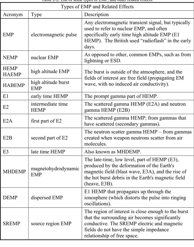
Table 2-2. List of some types of EMP, and other related effects. Types of EMP and Related Effects

Acronym Type Description

EMP electromagnetic pulse

Any electromagnetic transient signal, but typically used to refer to nuclear EMP, and often

specifically early time high altitude EMP (E1 HEMP). The British used “radioflash” in the early days.

NEMP nuclear EMP As opposed to other, common EMPs, such as from _{lightning or ESD.} HEMP

HAEMP high altitude EMP HABEMP high altitude burst _EMP

The burst is outside of the atmosphere, and the fields of interest are free field (propagating EM wave, with no induced air conductivity). E1 early time HEMP The prompt gamma part of HEMP. E2 intermediate time

HEMP

The scattered gamma HEMP (E2A) and neutron gamma HEMP (E2B)

E2A first part of E2 The scattered gamma HEMP; from gammas that _{have scattered (secondary gammas).} E2B second part of E2

The neutron scatter gamma HEMP – from gammas created when weapon neutrons scatter from air molecules.

E3 late time HEMP Also known as MHDEMP.

MHDEMP magnetohydrodynamic EMP

The late-time, low level, part of HEMP (E3), produced by the deformation of the Earth's magnetic field (blast wave, E3A), and the rise of the hot burst debris in the Earth's magnetic field (heave, E3B).

DEMP dispersed EMP E1 HEMP that propagates up through the ionosphere (which distorts the pulse into ringing oscillations).

SREMP source region EMP

The region of interest is close enough to the burst that the surrounding air becomes significantly conductive. The SREMP electric and magnetic fields do not have the simple impedance relationship of free space.

(Table 2-2 continued)

Types of EMP and Related Effects (continued) Acronym Type Description

SGEMP system generated _EMP

This EMP is driven by currents produced by the interaction of the burst's radiative particles with the structure of interest itself (as opposed to interactions with the air and ground, which produce SREMP fields). Because SREMP, when present, overshadows it, SGEMP is of most concern in the upper

atmosphere (little air) for external fields, and inside systems (see IEMP).

IEMP internal EMP

This is SGEMP produced inside a structure. Electrons emitted inside the structure, due to its interaction with the nuclear particles, create the currents and conductivity which produce internal electromagnetic energy – which has easier access to vulnerable electrical components.

NIL nuclear induced _lightning

For some surface burst nuclear tests there was lightning around the edge of the nuclear fireball – where only hardened buried structures would be expected to survive the blast anyway.

LEMP lightning EMP

A direct lightning strike could put very high currents onto a system. Also, a nearby strike produces an EM propagating pulse. However, the spatial region exposed to high fields is limited.

ESD electrostatic discharge

This is similar to a mini lightning strike – a direct discharge, created by a human, puts current onto the system, and propagating EM fields are generated. HIRF high intensity _{radiated fields} High level EM fields, such as from being close to a _{strong radar.}

IEMI

intentional electromagnetic interference

This is intentional malicious generation of

electromagnetic energy, so as to introduce noise or signals into electrical and electronic systems, and thus disrupt, confuse, or damage the systems for terrorist or criminal purposes.

HPM high power microwave

Concerned with narrowband EM environments that involve high signal levels. This can include IEMI, and HIRF, for example.

TREE

transient radiation effects on

electronics

This is generally not an EM field, but involves solid state physics effects of nuclear output particles (gamma, x ray, neutron, etc.) striking the active regions inside electronic devices, and causing upset or damage.

2.5 Parameters That Control E1 HEMP

To help understand E1 HEMP, it is useful to know what parameters have to be assigned values in order to make an E1 EMP calculation. Table 2-3 lists the parameters – the set is fairly short. They include characterization of the gamma and x-ray outputs for the burst. For the x rays it is only the high-energy ones that are important. The other parameters are geometry – placement of the burst and the observer.

Table 2-3. List of E1 HEMP input parameters. These parameters have to be given values in order to make an E1 HEMP environment calculation.

E1 HEMP Calculation Inputs Parameter Categories Parameters

Gammas Time evolution of gamma emission spectrum Weapon _{High energy x}

rays

Time evolution of high-energy x-ray emission spectrum

Burst location Latitude, longitude, altitude Geometry

Observer location Latitude, longitude (altitude if aircraft)

First consider the geometry factors. The burst location has to be given: latitude, longitude, and altitude; and then the same location information for the observer. As a simplification, traditionally the observer has just been assumed to be at sea level – accounting for topology would typically be more of a complication than it would be worth for the small effect on the magnitude of the incident E1 HEMP. Thus, observer altitude is usually not a required input. However, if one is concerned with aircraft, then altitude could be high enough to be significant – including the fact that the exposed region is larger, because rays above the tangent can expose more air space. For this document on the electric power system, however, the observer altitude can be ignored. The important aspects of geometry are:

1. Setting the intensity level – the 1/r2 spherical fall-off for the gammas to the source region, and for the EM wave power from there to the observer.

2. Setting the air density profile along the burst-observer ray. Shallower angles through the atmosphere (closer to tangent) mean lower, wider (and with less high frequency) pulses.

3. Setting the “source point” position, and so the geomagnetic field intensity and direction. The basic driver for E1 HEMP is given by the relative angle between the geomagnetic field lines and the burst-observer ray line (at the source points). 4. Determining the incident angle and polarization of the incident E1 HEMP at the

observer point.

All the geometry calculations involve straight-forward geometry and vector formulas. Gammas (more correctly, gamma rays) and x rays are both just photons – the same as other electromagnetic radiation (radio waves, visible light, infra-red, ultra-violet, etc.). Formally, gammas come from nuclear reactions (such as fission and fusion), while x rays

come from electron transitions in atoms. Typically, gammas have energies of several MeVs. Most of the burst output energy is in x-ray energy, but concentrated toward lower energies. (For an air burst, these x rays are quickly absorbed by the air, within a short distance, and they help generate the “fireball”.) For E1 HEMP the interest is only in the high-energy tail of the x-ray spectrum – tens of keV (but then just to a much less extent than the interest in the gammas).

As noted in the table, for E1 HEMP calculations the gamma spectrum must be given, along with the time waveform of the gamma emission. It is often assumed that the time and spectral variations are independent – the shape of the spectrum is always the same, just the total emission varies with the given time waveform. However, generally the spectrum does change with time, and for the best quality calculations the input data should give a separate time waveform for each gamma energy in its spectrum data.

In the early days of E1 HEMP calculational efforts, the x rays tended to be ignored. Most of the x-ray output is at low energies, and they are easily absorbed by the atmosphere. However, there are some x rays at much higher energies, such as 10 keV or more. For these photons we need the same information as for the gammas – time evolution of the spectrum (a time waveform for each energy in the spectrum data).

Two factors are important for the x rays:

1. X rays contribute little to generating E1 HEMP (they do not add much to the current source); their effect is mostly in generating air conductivity. So they tend to lower the peak of the E1 HEMP.

2. The burst output x rays tend to be delayed relative to the gammas.

Thus, if we ignore the x rays, we could over-predict the E1 HEMP field level. As the E1 HEMP is rising up from the currents produced by the gammas, the air conductivity may suddenly increase from the x rays, and the E1 rise will be halted. Thus the E1 HEMP peak value can be affected by both the gamma rays and the x rays.

It is important to note what is not important for E1 HEMP: 1. Kinetic energy.

2. Neutron output.

3. Low energy x rays (most of the weapon output energy) 4. Device yield.

It should also be noted that device yield cannot even be used indirectly to calculate the E1 HEMP. It is not possible to calculate the needed gamma and x-ray parameters from a given value of yield. There can be variations from one weapon design to the next in terms of the gamma and high energy x-ray parameters that are important for E1 HEMP. Some EMP calculations, such as source region EMP, need weather parameters – air density and water vapor content (from the humidity and temperature). These, especially considering large possible variations in water vapor content, affect the air chemistry (air conductivity) significantly. However, at very high altitudes these are not very important – there is not as much “weather” variation, and the water vapor content is very low.

2.6 HOB Variation

Note that the burst is described as being exoatmospheric – above the atmosphere. Except for various effects that can occur on satellites and very long range communications, the nuclear burst may not produce any other effects on man except through its HEMP. There is no exact criterion for HOB (height of burst) that qualifies for HEMP; however HEMP varies with HOB, as shown by the sample results in Figure 2-6. The average result (violet line) is averaged over the full exposed region, which is larger for higher HOB. For each weapon there is an optimum burst height to produce the maximum peak HEMP E field – usually somewhat less than 100 km. As one goes lower in HOB, the peak HEMP E eventually falls, and starts falling significantly when the burst locations gets into the atmosphere – typically we might ignore E1 HEMP when the HOB gets below about 20 km (again, an approximate altitude). Going to altitudes above the peak HOB, the peak HEMP E falls gradually, so that there might be some E1 HEMP when the burst is greater than many multiples of 100 km. Again, the exact details of the HOB variation (and other variations, such as with observer position) depend on the burst (the weapon parameters).

Figure 2-6. Sample E1 HEMP HOB variation. This shows the HOB variation, for a typical device, for the highest E1 peak seen over the full exposed region (red line), and for the average E1 Peak – averaged over all the exposed area. The E1 peak levels are plotted as a fraction of the absolute maximum E1 HEMP for all burst heights (it occurs about HOB=75 km in this case).

2.7 Exposed Region

However, besides the variation of the maximum E peak with HOB, there is also a variation in the area coverage – the amount of the Earth’s surface that is exposed to the E1 HEMP. This is simply determined by geometry – a given point on the Earth will be illuminated by E1 HEMP if it is within line-of-sight of the burst location. (For such determinations, for simplicity, the Earth is usually just assumed to be a sphere, ignoring topography and the Earth’s slight ellipsoid shape.) Figure 2-7 plots the radius of the exposed region versus burst height, and Figure 2-8 plots the area. Figure 2-9 shows area coverage for a burst over the U.S., for several burst heights.

As can be seen, a very large area is exposed to the E1 HEMP. Going higher (HOB higher) increases the area coverage, however, note that the ground range increase is sub-linear with HOB – the area coverage is approximately sub-linear in burst height. Also, the E1 HEMP strength tends to have its maximum for HOBs below 100 km, and so above that the extra area coverage for higher HOB comes at the expense of lower field levels.

Figure 2-8. E1 HEMP exposed region area versus burst height. The area is given in million of square kilometers (left axis) or square miles (right axis). The continental U.S. has an area of about 8.0 million square kilometers (3.1 million square miles).

Figure 2-9. Samples of E1 HEMP exposed regions for several heights. The red circles show the exposed regions for the given burst heights, for a nuclear burst over the central U.S.

2.8 E1 HEMP Geometry Features

There are a few common geometric features for a “smile” diagram. Figure 2-10 shows a north-south cut cross-section through a burst point in the northern hemisphere (all results shown in this report are for the northern geomagnetic hemisphere, and many results are shown for a burst over the central U.S.). The view is from the west, looking east, with the north to the left and the south to the right. This figure shows the three special points, and the tangents. The rays originating at the burst and that are tangent to the Earth’s surface define the maximum extent of the E1 HEMP exposure region, as discussed in the previous subsection.

Ground Zero (GZ) is the point directly below the burst – the observer ray goes straight down. This is the center of the smile diagram. Also, often observer points are located in terms of “ground range” – this is the distance, along the Earth’s surface, from GZ to the observer (a full location determination would then also require the observer’s azimuthal angle, such as measured clockwise from the north direction).

The red region in the atmosphere is the “source region” – its boundary depends on how we want to define it, but could be assumed to be, for example, the region between 20 and 40 km in altitude. The GZ ray goes through the source region most directly, and for the tangent point the ray is more oblique, taking a longer path in going through the source region layer. (We can also see that the spherical divergence effect – 1/r2 fall off – means the level of the gammas reaching the source region is less as we go out from the GZ point.)

Figure 2-10. Explanation of smile diagram variation along the center north/south line. This is a cut through the center, with north to the left, and south to the right, for a northern hemisphere burst. (For the southern hemisphere the null point is on the south, and the max point to the north.)

The bottom edge of the source region could be defined relative to the “breakaway point”. On the ray from the burst to the observer, the level of the gammas decrease along its path through the source region, and the level of the E1 HEMP increases. At some point the gammas are too weak to contribute much more to increasing the level of the E1 HEMP, nor to generated high enough air conductivity to erode away much of the E1 HEMP field. This is essentially the bottom edge of the source region. This is called the breakaway point – for points further down the ray the E1 HEMP is now a free wave, with no more effects from the sources and conductivities of the source region. This is really an arbitrary point, because the gamma effects do not suddenly stop at any point, but decrease smoothly (but sharply) with increasing air density. Often some criterion is used to define breakaway, such as the condition

⎟ ⎟ ⎠ ⎞ ⎜ ⎜ ⎝ ⎛ σ < σ

σ _{in conductiveair}

dz dE E ion to approximat an is side hand right the Z 2 dz d _o

where σ is the air conductivity, E is the electric field (both vary with time), and Zo is the

impedance of free space (about 376.7 ohms). (The right hand side is the attenuation distance of EM waves for σ«ωεo.) This condition says that the conductivity is falling

faster (relatively) with lower altitude than the relative fall in the E field due to conductivity. Generally we would want to take any E1 HEMP calculations to slightly lower altitudes. (Although often a simpler lower altitude criterion is used – assuming the bottom of the source region has been hit when the calculated rE product, E times distance from the burst, did not change significantly from the previous calculational position.) The other two special positions in Figure 2-10 are related to the geomagnetic field. The “null point” is where the observer ray and geomagnetic field lines are parallel. For this point the E1 HEMP is very low (ideally it would be zero). On the opposite side of GZ is the “max field point” (or “max point” for short). This term has been used to name the location on the smile diagram where the E1 HEMP has its maximum peak level. There are two effects involved in this – one is that the most direct rays through the atmosphere generally produce the highest E1 levels, and so this would favor the GZ ray. However, the second effect is the angle at which the observer ray crosses the geomagnetic field lines – favoring the point at which they are at right angles. This point could be called the “geomagnetic max point”. Note that the max field point depends on both the device and geometry, while the geomagnetic max point only depends on geometry.

For the northern hemisphere, generally the max field point is a little north of the geomagnetic max point – pulled away from the point of being at right angle to BGeo by

the better angle through the atmosphere nearer to GZ. However, there is a third effect that also sometimes comes into play. This involves the breakaway point. For very large gamma outputs and very lower burst heights, the breakaway altitude may be pushed very low, especially for straight down rays. At such low altitudes the Compton electrons have shorter life times, thus less turning in the geomagnetic field and so less total source current to generate the E1 HEMP. Thus, for such cases (large gamma output, very low HOB), the atmosphere angle variation might not be best straight down – there it might actually be significantly suppressed. In that case the max field point might vary from the

usual position of being a little north of the geomagnetic max point, and actually be south of the geomagnetic max point, especially for lower geomagnetic latitudes.

Note that for this report we will often mean “geomagnetic max point” when we use the “max point” term. The geomagnetic max point depends only on the geometry – the burst location (latitude, longitude, and height) – while the actual maximum field point, typically slightly to the south of GZ for a northern hemisphere burst, also depends on the characteristics of the nuclear explosion, and so varies from weapon to weapon.

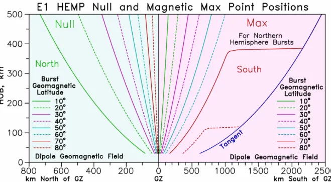
Figure 2-11 shows two plots – it gives the ground range from GZ to the null point (on the left) and geomagnetic max point (on the right) versus HOB (burst height), for various geomagnetic latitudes. (For example the position 40oN, 100oW, in the central U.S., has a geomagnetic dip angle of 67.55o, and geomagnetic latitude of about 50.43oN.) Different horizontal axis scalings are used for the two sides of the figure. The solid green line (to the left on both sides of the plot) is for the 10oN geomagnetic latitude positions, and then higher latitudes (closer to the geomagnetic poles) lines are to the right, up to the dashed red line for 80oN. The null point is always near GZ – the farthest it is away is for a burst near the equator. As seen, it is about 700 km away from GZ, out of the maximum E1 radius of about 2400 km, for a 500 km HOB. (The blue line on the right side gives the tangent ground range.) For the geomagnetic max point the variation is the opposite – the maximum range from GZ is for the higher latitudes; and it gets so far out that for the 75oN and 80oN cases the max point gets out to the tangent point and beyond for higher burst heights (the red lines go out to the blue line).

Figure 2-11. Positions of two special E1 HEMP points versus burst height. The position of the null point is on the left side of plot, and the geomagnetic max point is on the right side of plot (different x axis scalings are used in the two sides). This is for an ideal dipole model of the Earth’s geomagnetic field. The lines are for 10o _{increments in geomagnetic latitude (solid green for 10}o _{above the equator, up to dashed red for 80}o_,

2.9 Incident and Total E1 HEMP Environments

Traditionally HEMP is given as the E field in the pulse that is traveling down to the Earth – the incident E field. Some effects are ignored, such as the elevation of the Earth surface at the observation point (the local topography), or small observer heights off the ground. (For aircraft at high altitudes, it is easy to account for the 1/r fall-off in E field to go back to an observer point that is far off the ground). A simple spherical Earth is generally assumed, and the incident field at sea level is given.

Also, very localized conditions are not accounted for in smile diagrams and typical HEMP calculations. For example, for points near the tangent, the shadowing effect of being in a deep canyon is not included. And there could be reflection effects, such as being near the side of a very large metal building. Also, long conductors – power lines, fences, railroad rails – can collect EM energy, and so enhance the HEMP for observers nearby. These are all ignored, generally because they are considered highly variable, or too random to include in a large area display such as a smile diagram. They are considered in performing detailed localized coupling calculations.

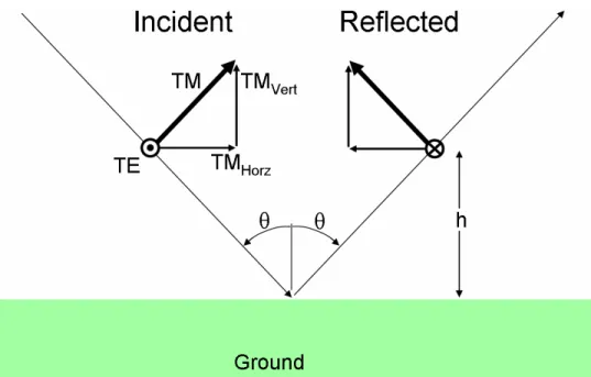
Some effects can be calculated, if the HEMP environment is known. For example, to go a step beyond the typical calculation of the HEMP, the reflection off the Earth surface can be accounted for. Consider an incident E1 HEMP, as shown in Figure 2-12. The plane perpendicular to the incident ray is shown (it tilts forward, as required by the downward angle of the ray). The E1 E field (and H field) must be in this plane – we have separated the E field into two terms, also in this plane. The transverse electric “TE” term is horizontal, the transverse magnetic “TM” term is normal to this, and “upward” – but it has a forward tilt corresponding to the plane’s tilt. Figure 2-13 shows a side view of this, for an observer position that is a small distance “h” above the ground. The incident wave is on the left, and the reflected on the right. Note that the horizontal terms (TE and TMHorz) change signs on reflecting, while the vertical term (TMVert) does not.

At the observer point the incident pulse will be seen, and then that pulse will go down to the surface and then back up, so that the observer will also see a reflected pulse. (We ignore the very slight difference in horizontal positions that goes with these two pulses – E1 HEMP does not vary over such small horizontal distances.) However, because of the signs of the reflections for each component, the reflected vertical component will add to the incident pulse, while the other components (horizontal) will tend to cancel the incident pulse. The time delay for the reflection is

θ =

∆ cos

c h 2

where “c” is the speed of light, “h” is the observer height above the ground, and θ is the incident ray angle from vertical. For several meter heights this offset time may be on the order of 10 nanoseconds (with large variation, depending on height and ground range from ground zero). Typical E1 HEMP pulses are tens of nanoseconds wide, so the reflection pulse comes back well within the time that the incident pulse is still present. The shorter the offset time (smaller observer height or closer to the tangent of the

exposed region), the more the total field seen is that of doubling the incident vertical field and canceling (zeroing out) the horizontal field.

Figure 2-12. Decomposing an incident E1 HEMP into two E field terms for reflection. E1 can be decomposed into the part with the E field horizontal and to the side (TE), and the other part (TM), which is upward in the plane perpendicular to the burst-observer ray. (This field orientation is appropriate for a westward ray.)

Figure 2-13. E1 HEMP Earth reflection. In this example the Earth is considered to be a perfect conductor. The previous discussion was for a perfect conductor, while the real Earth is not perfect. The higher the conductivity, the more perfect it is. The calculation of reflections for imperfect ground is straight forward, but more complex. The reflection coefficients for the three terms all become functions of frequency, and an E1 HEMP’s frequency content is very wide. As an approximation for picturing this, we can think of skin depth, defined as

µ σ π = δ

f 1

.

In simple terms, this is the distance that an EM wave of frequency “f” penetrates into a ground of conductivity “σ” (and permeability “µ”, but this typically does not vary much from place to place). We can think of the reflection point not being at the Earth’s surface, but further down into the ground, as given by the skin depth. Note however that the lower the frequency component, the further down the reflection surface is. Thus, the total field is very complex. (This skin depth effect is also why E1 reflections deal mostly with the soil near the Earth’s surface, while the E3 HEMP is concerned with the conductivity much deeper into the Earth.)

As noted, E1 HEMP has a very wide range of frequencies (this will be shown shortly). The parameters that govern the EM response of soil tend to also vary significantly with frequency. As frequency increases, the conductivity increases, and the permittivity decreases. This further complicates the reflection process. To account for this there has to be data available for the frequency dependence of soil, and we would expect this to vary with soil type. Another complication is that for many soils, the water content has a very significant effect on its parameter values, so it may depend upon what the recent weather has been. For some EMP studies a “universal soil” model has often been used, in which the water content is a single variable that roughly determines the soil frequency variations.

Besides the reflection from a flat, homogeneous ground surface, there may be other objects that cause reflections, or other electromagnetic effects that might affect the total E1 HEMP signal seen at a point. This includes reflection from nearby buildings, for example. Also, long conductors can be important (a fence, railroad, or power line) if nearby, because the E1 HEMP can cause large currents to flow, and there are EM fields associated with such large coupled currents.

2.10 Generic E1 HEMP Environment

A given set of input parameters, including time waveforms for the burst outputs, will produce a specific E1 HEMP waveform. Typically such waveforms rise up quickly, and then fall somewhat slower. Many such E1 HEMP waveforms that have been calculated from computer models, and many generic E1 HEMP standard waveforms have been created. They are attempts to capture the characteristics of E1 HEMP waveforms, in general, in a convenient analytic form. Besides the waveform used, they generally also specify the signal amplitude. Because of “saturation” (the fact that induced air conductivity limits the growth in the E1 HEMP amplitude) it makes some sense to have a single amplitude level. However, this can also be done because the specified waveform is typically meant to be worse case – the highest peak signal that is likely to be observed. We have also mentioned that the waveshape is faster and narrower near ground zero, and becomes slower and wider out near the tangent. Thus, one waveform cannot represent such a range of shapes, and some compromise must be applied. Several approaches may

be used. Since the highest peaks are associated with close-in observers, the fast pulse might be emphasized. Or the rise time may be set by the fast pulse, and the width set by the slow pulse. This might be considered as “drawing an envelope around all possible pulses”.

Often an E1 HEMP specification also gives a frequency spectrum (Fourier transform). This might simply be the transform of the given waveform. However, again there is some variation in spectra – with near-in points going farther out to higher frequencies, but points farther out toward the tangent having more low frequency energy. So another approach is to have a frequency specification that is unconnected to the given waveform – one approach is to use an envelope of all possible spectra.

Most generic E1 HEMP waveforms use one of these two forms t

t _e e−β − −α or t t _e e 1 α − β ₊

with an appropriate provision for when to start the waveform. The first equation naturally starts at zero time, where it has the value of zero. The second equation never goes to zero, and we have to pick some arbitrary time point at which we say the E1 HEMP waveform starts. The α sets the pulse rise, and β the fall.

One generic waveform is given by the IEC (“Electromagnetic compatibility (EMC) – Part 2: Environment – Section 9: Description of HEMP environment – Radiated disturbance, Basic EMC publication”, IEC 61000-2-9, February 1996, International Electrotechnical Commission, Geneva, Switzerland):

(

)

E _{b t a t}

1 01

1 _{1 1}

1 7 1 1 8 1 b a b 1 1 1 1 1 1 01 s 10 4 b s 10 6 a 3 . 1 b a b a a k m / V 000 , 50 E 1 1 1 − − ⎟⎟ ⎠ ⎞ ⎜⎜ ⎝ ⎛ − × = × = = ⎟⎟ ⎠ ⎞ ⎜⎜ ⎝ ⎛ ⎟⎟ ⎠ ⎞ ⎜⎜ ⎝ ⎛ − = = with spectrum

(

)(

)

− =

=

ω

_∫

j b j a b a k E dt e ) t ( E ) ( E 1 1 1 1 1 01 t j 1

1 .

Table 2-4 summarizes some characteristics of this generic E1 HEMP signal. By construction, is has a peak of 50 kV/m. The peak power is very high, but the total energy (approximately peak power times pulse width) is modest. The pulse rises in a few nanoseconds, and has a pulse width of about 23 nanoseconds. The spectrum extends well above 100 MHz.

Table 2-4. Characteristics of the IEC E1 HEMP waveform. IEC E1 HEMP Waveform Properties

Characteristic Value Waveform peak Epeak =50,000V/m

Spectrum peak Elowfreq =0.00152V/m/Hz

Waveform peak power P_peak =6.64×106 W/m2

Spectrum peak power P_lowfreq =6.11×10−9 W/m2/Hz Total energy W_total =0.115J/m2

Time of peak tpeak =4.84ns Rise time, 10% to 90% of peak t₁₀₋₉₀ =2.47ns Pulse width, full width at half maximum FWHM=23.0ns Pulse width, total energy over peak power Wtotal/Ppeak =17.3ns Spectrum width, total energy over peak

spectrum power Wtotal/Plowfreq =18.8MHz

To get a feeling for this E1 HEMP signal, consider another EM signal – a FM radio transmission at 100 MHz. Assume the transmitted power is 10,000 watts (RMS), and we are receiving the signal close by, at a distance of 1 mile (1.61 km). For a crude estimate, assume a transmitting antenna gain of 2 (2 in power). Then the peak power at the 1 mile range is 1.23 mW/m2, and the peak electric field is 0.68 V/m. Thus, this signal is smaller than the E1 HEMP electric field peak by a factor of 73,500 – or a factor of 5.4×109 _{in power (97.3 dB). Figure 2-14 shows the IEC E1 HEMP waveform, compared}

to the FM radio signal – scaled up to the same amplitude. We can also see that the rise of the E1 pulse is similar to the rise of a cycle of the FM signal, and so we can see that the E1 HEMP does have signal content up to 100 MHz. Figure 2-15 shows the actual spectrum of the E1 HEMP waveform.

Certainly the E1 HEMP signal is much larger than the FM radio signal. However, the E1 HEMP energy density is modest - 0.114 Joules/m2. By contrast, about every 3.1 minutes the FM radio signal delivers the same amount of energy density (of course the E1 HEMP delivers its energy in a few tens of nanoseconds, and over a much larger area). This is an energy density – the amount of energy going by through an area of a square meter. In general it would also be about the amount of energy picked up by a wire antenna about a meter long. Coupling collection areas can vary quite a bit, of course. For example, a long wire could collect significantly more than 0.114 Joules.

Figure 2-14. Sample E field signals for E1 HEMP and FM radio. The parameters for the FM radio signal are listed in the figure. Note, however, that the FM signal has been multiplied by 73,500, to get it up to the same amplitude as the HEMP signal. The FM signals goes on forever (essentially), while the E1 HEMP signal is transient, and very short-lived.

Figure 2-15. Spectrum of the idealized E1 HEMP E field signal. This is the spectrum (magnitude of the Fourier transform) for the signal shown in Figure 2-14. This sample E1 HEMP pulse is flat up to about 10 MHz, and then it starts falling for higher frequencies.