An Evaluator for Human Pose Estimators
Nataraj Jammalamadaka‡, Andrew Zisserman†, Marcin Eichner§, Vittorio Ferrariz, and C. V. Jawahar‡
‡
IIIT-Hyderabad,†University of Oxford,§ETH Zurich,zUniversity of Edinburgh
Abstract. Most current vision algorithms deliver their output ‘as is’, without indicating whether it is correct or not. In this paper we proposeevaluator algo-rithmsthat predict if a vision algorithm has succeeded. We illustrate this idea for the case of Human Pose Estimation (HPE).
We describe the stages required to learn and test an evaluator, including the use of an annotated ground truth dataset for training and testing the evaluator (and we provide a new dataset for the HPE case), and the development of auxiliary features that have not been used by the (HPE) algorithm, but can be learnt by the evaluator to predict if the output is correct or not.
Then an evaluator is built for each of four recently developed HPE algorithms using their publicly available implementations: Eichner and Ferrari [5], Sappet al.[16], Andrilukaet al.[2] and Yang and Ramanan [22]. We demonstrate that in each case the evaluator is able to predict if the algorithm has correctly estimated the pose or not.
1
Introduction
Computer vision algorithms for recognition are getting progressively more complex as they build on earlier work including feature detectors, feature descriptors and classi-fiers. A typical object detector, for example, may involve multiple features and multiple stages of classifiers [7]. However, apart from the desired output (e.g. a detection win-dow), at the end of this advanced multi-stage system the sole indication of how well the algorithm has performed is typically just the score of the final classifier [8, 18].
The objective of this paper is to try to redress this balance. We argue that algorithms
shouldandcanself-evaluate. They should self-evaluate because this is a necessary
re-quirement for any practical systems to be reliable. That they can self-evaluate is demon-strated in this paper for the case of human pose estimation (HPE). Such HPE evaluators can then take their place in the standard armoury of many applications, for example removing incorrect pose estimates in video surveillance, pose based image retrieval, or action recognition.
In general four elements are needed to learn an evaluator: a ground truth annotated database that can be used to assess the algorithm’s output; a quality measure comparing the output to the ground truth; auxiliary features for measuring the output; and a classi-fier that is learnt as the evaluator. After learning, the evaluator can be used to predict if the algorithm has succeeded on new test data, for which ground-truth is not available. We discuss each of these elements in turn in the context of HPE.
For the HPE task considered here, the task is to predict the 2D (image) stickman layout of the person: head, torso, upper and lower arms. The ground truth annotation in the dataset must provide this information. The pose quality is measured by the differ-ence between the predicted layout and ground truth – for example the differdiffer-ence in their angles or joint positions. The auxiliary features can be of two types: those that are used or computed by the HPE algorithm, for example max-marginals of limb positions; and those that have not been considered by the algorithm, such as proximity to the image boundary (the boundary is often responsible for erroneous estimations). The estimate given by HPE on each instance from the dataset is then classified, using a threshold on the pose quality measure, to determine positive and negative outputs – for example if more than a certain number of limbs are incorrectly estimated, then this would be deemed a negative. Given these positive and negative training examples and both types of auxiliary features, the evaluator can be learnt using standard methods (here an SVM). We apply this evaluator learning framework to four recent publicly available meth-ods: Eichner and Ferrari [5], Sappet al.[16], Andrilukaet al.[2] and Yang and Ra-manan [22]. The algorithms are reviewed in section 2. The auxiliary features, pose qual-ity measure, and learning method are described in section 3. For the datasets, section 4, we use existing ground truth annotated datasets, such asETHZ PASCAL Stickmen[5]
andHumans in 3D[4], and supplement these with additional annotation where
neces-sary, and also introduce a new dataset to provide a larger number of training and test examples. We assess the evaluator features and method on the four HPE algorithms, and demonstrate experimentally that the proposed evaluator can indeed predict when the algorithms succeed.
Note how the task of an HPE evaluator is not the same as that of deciding whether the underlying human detection is correct or not. It might well be that a correct detection then leads to an incorrect pose estimate. Moreover, the evaluator cannot be used directly as a pose estimator either – a pose estimator predicts a pose out of an enormous space of possible structured outputs. The evaluator’s job of deciding whether a pose is correct is different, and easier, than that of producing a correct pose estimate.
Related work. On the theme of evaluating vision algorithms, the most related work
to ours is Mac Aodha et al.[12] where the goal is to choose which optical flow al-gorithm to apply to a given video sequence. They cast the problem as a multi-way classification. In visual biometrics, there has also been extensive work onassessor al-gorithms which predict an algorithm’s failure [17, 19, 1]. These assess face recognition algorithms by analyzing the similarity scores between a test sample and all training im-ages. The method by [19] also takes advantage of the similarity within template imim-ages. But none of these explicitly considers other factors like imaging conditions of the test query (as we do). [1] on the other hand, only takes the imaging conditions into account. Our method is designed for another task, HPE, and considers several indicators all at the same time, such as the marginal distribution over the possible pose configurations for an image, imaging conditions, and the spatial arrangement of multiple detection win-dows in the same image. Other methods [20, 3] predict the performance by statistical analysis of the training and test data. However, such methods cannot be used to predict the performance on individual samples, which is the goal of this paper.
0.084 5.02
0.075 11.66
0.032 20.35 Max
Var
Unimodal Multi modal Large spread
Max Var
Max Var
Fig. 1:Features based on the output of HPE.Examples of unimodal, multi-modal and large spread pose estimates. Each image is overlaid with the best configuration (sticks) and the poste-rior marginal distributions (semi-transparent mask). ‘Max’ and ‘Var’ are the features measured from this distribution (defined in the text). As the distribution moves from peaked unimodal to more multi-modal and diffuse, the maximum value decreases and the variance increases.
2
Human pose estimation
In this section, we review four human pose estimation algorithms (HPE). We also re-view the pictorial structure framework, on which all four HPE techniques we consider are based on.
2.1 Upper body detection
Upper body detectors (UBD) are often used as a preprocessing stage in HPE pipelines [5, 16, 2]. Here, we use the publicly available detector of [6]. It combines an upper-body detector based on the part-based model of [8] and a face detector [18]. Both components are first run independently in a sliding window fashion followed by non-maximum sup-pression, and output two sets ofdetection windows(x, y, w, h). To avoid detecting the same person twice, each face detection is then regressed into the coordinate frame of the upper-body detector and suppressed if it overlaps substantially with any upper-body detection. As shown in [6] this combination yields a higher detection rate at the same false-positive rate, compared to using either component alone.
2.2 Human pose estimation
All methods we review are based on the pictorial structure framework. An UBD is used to determine the location and scale(x, y, w, h)of the person for three of the HPE methods we consider [5, 16, 2]. Pose estimation is then run within anextended
detec-tion windowof width and height2wand2.5hrespectively. The method of Yang and
Ramanan [22] is the exception. This runs directly on the image, without requiring an UBD. However, it generates many false positive human detections, and these are re-moved (in our work) by filtering using an UBD.
Pictorial structures (PS). PS [9] model a person’s body parts as conditional random
field (CRF). In the four HPE methods we review, partsliare parameterized by location
Fig. 2:Human pose estimated based on an in-correct upper-body detection: a typical exam-ple of a human pose estimated in a false posi-tive detection window. The pose estimate (MAP) is an unrealistic pose (shown as a stickman, i.e. a line segment per body part) and the poste-rior marginals (PM) are very diffuse (shown as a semi-transparent overlay: torso in red, upper arms in blue, lower arms and head in green). The pose estimation output is from Eichner and Ferrari [5].
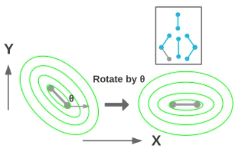
X Y
θ
Rotate by θ
Fig. 3:Pose normalizing the marginal distri-bution.Marginal distribution (contour diagram in green) on the left ispose normalizedby rotat-ing it by an angleθ of the body part (line seg-ment in grey) to obtain the transformed distribu-tion on the right. In the inset, the pertinent body part (line segment in grey) is displayed as a con-stituent of the upper body.
expP
(i,j)∈EΨ(li, lj) +PiΦ(I|li)
. The unary potentialΦ(I|li)evaluates the local
image evidence for a part in a particular position. The pairwise potentialΨ(li, lj)is a
prior on the relative position of parts. In most works the model structureEis a tree [5, 9, 14, 15], which enables exact inference. The most common type of inference is to find the maximum a posteriori (MAP) configurationL∗ = arg max
LP(L|I). Some works
perform another type of inference, to determine the posterior marginal distributions over the position of each part [5, 14, 11]. This is important in this paper, as some of the features we propose are based on the marginal distributions (section 3.1). The four HPE techniques [5, 16, 2, 22] we consider are capable of both types of inference. In this paper, we assume that each configuration has six parts corresponding to the upper-body, but the framework supports any number of parts (e.g. 10 for a full body [2]).
Eichner and Ferrari [5]. Eichneret al. [5] automatically estimate body part appearance
models (colour histograms) specific to the particular person and image being analyzed, before running PS inference. These improve the accuracy of the unary potential Φ, which in turn results in better pose estimation. Their model also adopts the person-generic edge templates as part ofΦand the pairwise potentialΨof [14].
Sappet al. [16]. This method employs complex unary potentials, and non-parametric data-dependent pairwise potentials, which accurately model human appearance. How-ever, these potentials are expensive to compute and do not allow for typical inference speed-ups (e.g. distance transform [9]). Therefore, [16] runs inference repeatedly, start-ing from a coarse state-space for body parts and movstart-ing to finer and finer resolutions.
Andriluka et al. [2]. The core of this technique lies in proposing discriminatively
trained part detectors for the unary potentialΦ. These are learned using Adaboost on shape context descriptors. The authors model the kinematic relation between body parts
using Gaussian distributions. For the best configuration of parts, they independently in-fer the location of each part from the marginal distribution (corresponding to the maxi-mum), which is suboptimal compared to a MAP estimate.
Yang and Ramanan [22]. This method learns unary and pairwise potentials using a
very effective discriminative model based on the latent-svm algorithm proposed in [8]. Unlike the other HPE methods which model limbs as parts, in this method parts cor-respond to the mid and end points of each limb. As a consequence, the model has18 parts. Each part is modeled as a mixture to capture the orientations of the limbs.
This algorithm searches over multiple scales, locations and all the part mixtures (thus implicitly over rotations). However, it returns many false positives. The UBD is used as a post-processing step to filter these out, as its precision is higher. In detail, all human detections which overlap less than50%with any UBD detection are discarded. Overlap is measured using the standard “intersection over union” criteria [7].
3
Algorithm evaluation method
We formulate the problem of evaluating the human pose estimates as classification into ‘success’ and ‘failure’ classes. First, we describe the novel features we use (section 3.1). We then explain how human pose estimates are evaluated. For this, we introduce a measure of quality for HPE by comparing it to a ground-truth stickman (section 3.2). The features and quality measures are then used to train the evaluator as a classifier (section 3.3)
3.1 Features
We propose a set of features to capture the conditions under which an HPE algorithm is likely to make mistakes. We identify two types of features: (i) based on the output of the HPE algorithm – the score of the HPE algorithm, marginal distribution, and best configuration of partsL∗; and, (ii) based on the extended detection window – its position, overlap with other detections, etc – these are features which have not been used directly by the HPE algorithm. We describe both types of features next.
1. Features from the output of the HPE. The outputs of the HPE algorithm consist of a marginal probability distribution Pi over(x, y, θ)for each body part i, and the
best configuration of partsL∗. The features computed from these outputs measure the spread and multi-modality of the marginal distribution of each part. As can be seen from figures 1 and 2, the multi-modality and spread correlate well with the error in the pose estimate. Features are computed for each body part in two stages: first, the marginal distribution is pose-normalized, then the spread of the distribution is measured by comparing it to an ideal signal.
The best configurationL∗, predicts an orientationθfor each part. This orientation is used to pose-normalize the marginal distribution (which is originally axis-aligned) by rotating the distribution so that the predicted orientation corresponds to thex-axis (illustrated in figure 3). The pose-normalized marginal distribution is then factored into three separatex,yandθspaces by projecting the distribution onto the respective axes. Empirically we have found that this step improves the discriminability.
A descriptor is then computed for each of the separate distributions which measure its spread. For this we appeal to the idea of a matched filter, and compare the distribution to an ideal unimodal one,P∗, which models the marginal distribution of a perfect pose estimate. The distributionP∗is assumed to be Gaussian and its variance is estimated from training samples with near perfect pose estimate. The unimodal distribution shown in figure 1 is an example corresponding to a near perfect pose estimate.
The actual feature is obtained by convolving the ideal distribution,P∗, with the measured distribution (after the normalization step above), and recording the maximum value and variance of the convolution. Thus for each part we have six features, two for each dimension, resulting in a total of36features for an upper-body. The entropy and variance of the distributionPi, and the score of the HPE algorithm are also used as
features taking the final total to36 + 13features.
Algorithm specific details: While the procedure to compute the feature vector is
essentially the same for all four HPE algorithms, the exact details vary slightly. For An-drilukaet al. [2] and Eichner and Ferrari [5], we use the posterior marginal distribution to compute the features. While for Sappet al. [16] and Yang and Ramanan [22], we use the max-marginals. Further, in [22] the pose-normalization is omitted as max-marginal distributions are over the mid and end points of the limb rather than over the limb itself. For [22], we compute the max-marginals ourselves as they are not available directly from the implementation.
2. Features from the detection window. We now detail the 10 features computed over the extended detection window. These consist of the scale of the extended detection window, and the confidence score of the detection window as returned by the upper body detector. The remainder are:
Two image features: the mean image intensity and mean gradient strength over the
extended detection window. These are aiming at capturing the lighting conditions and the amount of background clutter. Typically HPE algorithms fail when either of them has a very large or a very small value.
Four location features: these are the fraction of the area outside each of the four image
borders. Algorithms also tend to fail when people are very small in the image, which is captured by the scale of the extended detection window. The location features are based on the idea that the larger the portion of the extended detection window which lies outside the image, the less likely it is that HPE algorithms will succeed (as this indicates that some body parts are not visible in the image).
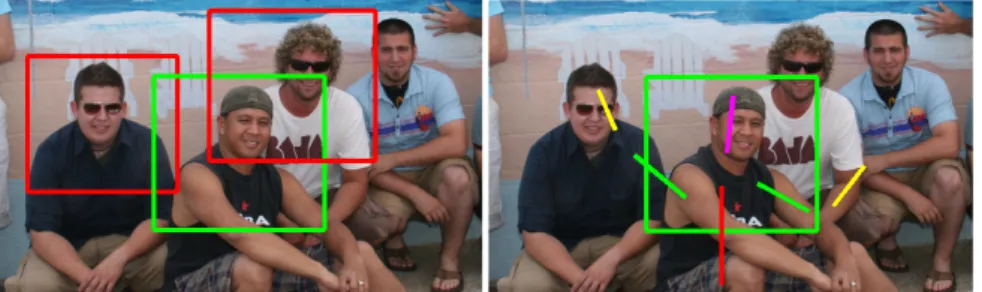
Two overlap features: (i) the maximum overlap, and (ii) the sum of overlaps, over all
the neighbouring detection windows normalized by the area of the current detection window. As illustrated in Figure 4 HPE algorithms can be affected by the neighbouring people. The overlap features capture the extent of occlusion by the neighbouring detec-tion windows. Overlap with other people indicates how close the they are. While large overlaps occlude many parts in the upper body, small overlaps also affect HPE perfor-mance as the algorithm could pick the parts (especially arms) from their neighbours.
While measuring the overlap, we consider only those neighbouring detections which have similar scale (between0.75and1.25times). Other neighbouring detections which are at a different scale typically do not affect the pose estimation algorithm.
Fig. 4: Overlap features.Left: Three overlapping detection windows. Right: the HPE output is incorrect due to interference from the neighbouring people. This problem can be flagged by the detection window overlap (output from Eichner and Ferrari [5]).
3.2 Pose quality measure
For evaluating the quality of a pose estimate, we devise a measure which we term the
Continuous Pose Cumulative error(CPC) for measuring the dissimilarity between two
poses. It ranges in[0,1], with 0 indicating a perfect pose match. In brief, CPC depends on the sum of normalized distances between the corresponding end points of the parts. Figure 5 gives examples of actual CPC values of poses as they move away from a ref-erence pose. The CPC measure is similar to thepercentage of correctly estimated body
parts(PCP) measure of [5]. However, CPC adds all distances between parts, whereas
PCP counts the number of parts whose distance is below a threshold. Thus PCP takes in-teger values in{0, . . . ,6}. In contrast, for proper learning in our application we require a continuous measure, hence the need for the new CPC measure.
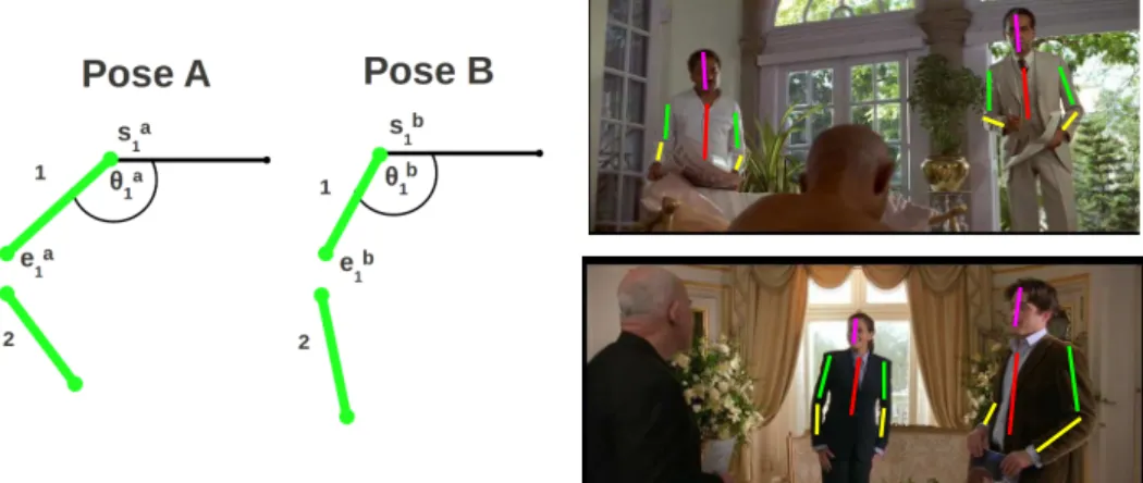
In detail, the CPC measure computes the dissimilarity between two poses as the sum of the differences in the position and orientation over all parts. Each pose is described byN parts and each partpin a poseAis represented by a line segment going from pointsa
pto pointeap, and similarly for pose B. All the coordinates are normalized with
respect to the detection window in which the pose is estimated. The angle subtended by
pisθa
p. With these definitions, theCP C(A, B)between two posesAandBis:
CP C(A, B) =σ
N
X
p=1 wp
sap−sbp
+
eap−ebp
2sa p−eap
!
with wp= 1 + sin
|θpa−θbp| 2
! (1)
whereσis the sigmoid function andθap−θpbis the relative angle between partpin pose
AandB, and lies in[−π, π]. The weightwpis a penalty for two corresponding parts
ofAandBnot being in the same direction. Figure 6 depicts the notation in the above equation.
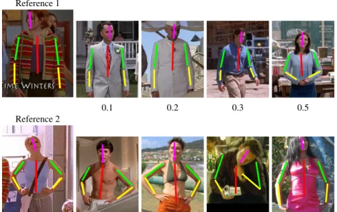
Reference 1
0.1 0.2 0.3 0.5
Reference 2
Fig. 5:Poses with increasing CPC.An example per CPC is shown for each of the two reference poses for CPC measures of 0.1, 0.2, 0.3 and 0.5. As can be seen example poses move smoothly away from the reference pose with increasing CPC, with the number of parts which differ and the extent increasing. For 0.1 there is almost no difference between the examples and the reference pose. At 0.2, the examples and reference can differ slightly in the angle of one or two limbs, but from 0.3 on there can be substantial differences with poses differing entirely by 0.5.
3.3 Learning the pose quality evaluator
We require positive and negative pose examples in order to train the evaluator for an HPE algorithm. Here a positive is where the HPE has succeeded and a negative where it has not. Given a training dataset of images annotated with stickmen indicating the ground truth of each pose, (section 4.1), the positive and negative examples are obtained by comparing the output of the HPE algorithms to the ground truth using CPC and thresholding its value. Estimates with low CPC (i.e. estimates close to the true pose) are the positives, and those above threshold are the negatives.
In detail, the UBD algorithm is applied to all training images, and the four HPE algorithms [5, 16, 2, 22] are applied to each detection window to obtain a pose estimate. The quality of the pose estimate is then measured by comparing it to ground truth using CPC. In a similar manner to the use of PCP [5], CPC is only computed for correctly localized detections (those with IoU>0.5). Detections not associated with any ground-truth are discarded. Since all of the HPE algorithms considered here can not estimate partial occlusion of limbs, CPC is set to 0.5 if the ground-truth stickman has occluded parts. In effect, the people who are partially visible in the image get high CPC. This is a means of providing training data for the evaluator that the HPE algorithms will fail on these cases.
Fig. 6: Pose terminology:For poses A and B corresponding partspare illustrated. Each part is described by starting pointsa
p, end pointea p and the angle of the partθa
pare also illustrated.
Fig. 7: Annotated ground-truth samples (stickman overlay) for two frames from the Movie Stickmen dataset.
A CPC threshold of0.3 is used to separate all poses into a positive set (deemed correct) and a negative set (deemed incorrect). This threshold is chosen because pose estimates with CPC below 0.3 are nearly perfect and roughly correspond to PCP = 6 with a threshold of 0.5 (figure 5). A linear SVM is then trained on the positive and negative sets using the auxiliary features described in section 3.1. The feature vector has59dimensions, and is a concatenation of the two types of features (49components based on the output of the HPE, and10based on the extended detection window). This classifier is the evaluator, and will be used to predict the quality of pose estimates on novel test images.
The performance of the evaluator algorithm is discussed in the experiments of sec-tion 4.2. Here we comment on the learnt weight vector from the linear SVM. The magni-tude of the components of the weight vector suggests that the features based on marginal probability, and location of the detection window, are very important in distinguishing the positive samples from the negatives. On the other hand, the weights of the upper body detector, image intensity and image gradient are low, so these do not have much impact.
4
Experimental evaluation
After describing the datasets we experiment on (section 4.1), we present a quantitative analysis of the pose quality evaluator (section 4.2).
4.1 Datasets
We experiment on four datasets. Two are the existingETHZ PASCAL Stickmen[5] and
Humans in 3D [4], and we introduce two new datasets, called Buffy2 Stickmen and
Movie Stickmen. All four datasets are challenging as they show people at a range of
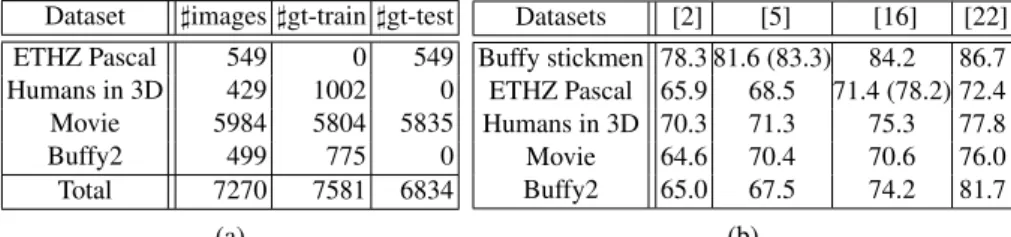
Dataset ]images]gt-train]gt-test
ETHZ Pascal 549 0 549
Humans in 3D 429 1002 0 Movie 5984 5804 5835
Buffy2 499 775 0
Total 7270 7581 6834 (a)
Datasets [2] [5] [16] [22] Buffy stickmen 78.3 81.6 (83.3) 84.2 86.7 ETHZ Pascal 65.9 68.5 71.4 (78.2) 72.4 Humans in 3D 70.3 71.3 75.3 77.8 Movie 64.6 70.4 70.6 76.0 Buffy2 65.0 67.5 74.2 81.7
(b)
Table 1:(a) Dataset statistics.The number of images and stickmen annotated in the training and test data.(b) Pose estimation evaluation.The PCP1of the four HPE algorithms (Andriluka et al.[2], Eichner and Ferrari [5], Sappet al.[16], Yang and Ramanan [22]) averaged over each dataset (at PCP threshold 0.5, section 3.2). The numbers in brackets are the results reported in the original publications. The differences in the PCPs are due to different versions of UBD software used. The performances across the datasets indicate their relative difficulty.
backgrounds. Buffy2 Stickmen is composed of frames sampled from episodes 2 and 3 of season 5 of the TV showBuffy the vampire slayer(note this dataset is distinct from the existing Buffy Stickmen dataset [11]). Movie Stickmen contains frames sampled from ten Hollywood movies (About a Boy, Apollo 13, Four Weddings and a Funeral, Forrest Gump, Notting Hill, Witness, Gandhi, Love Actually, The graduate, Groundhog
day).
The data is annotated with upper body stickmen (6 parts: head, torso, upper and lower arms) under the following criteria: all humans who have more than three parts visible are annotated, provided their size is at least 40 pixels in width (so that there is sufficient resolution to see the parts clearly). For near frontal (or rear) poses, six parts may be visible; and for side views only three. See the examples in figure 7. This fairly complete annotations includes self occlusions and occlusions by other objects and other people.
Table 1a gives the number of images and annotated stickmen in each dataset. As
atraining setfor our pose quality evaluator, we take Buffy2 Stickmen, Humans in 3D
and the first five movies of Movie Stickmen. ETHZ PASCAL Stickmen and the last five movies of Movie Stickmen form thetest set, on which we report the performance of the pose quality evaluator in the next subsection.
Performance of the HPE algorithms. For reference, table 1b gives the PCP performance
of the four HPE algorithms. Table 2 gives the percentage of samples where pose is estimated accurately, i.e. the CPC between the estimated and ground-truth stickmen is
<0.3In all cases, we use the implementations provided by the authors [5, 16, 2, 22] and all methods are given the same detection windows [6] as preprocessing. Both measures agree on the relative ranking of the methods: Yang and Ramanan [22] performs best, followed by Sappet al. [16], Eichner and Ferrari [5] and then by Andrilukaet al. [2]. This confirms experiments reported independently in previous papers [5, 16, 22]. Note
1We are using the PCP measure as defined by the source code of the evaluation protocol in [5],
Dataset [2] [5] [16] [22] Train 8.5 10.7 11.6 18.5 Test 9.9 11.1 12.0 16.5 Total 9.1 10.9 11.8 17.6
Table 2: Percentage of accurately estimated poses.The table shows the percentage of sam-ples which were estimated accurately (CPC<
0.3) on the training and test sets, as well as over-all, for the four HPE algorithms (Andrilukaet al.[2], Eichner and Ferrari [5], Sappet al.[16], Yang and Ramanan [22]). These accurate pose estimates form the positive samples for training and testing the evaluator.
CPC 0.2 CPC 0.3 CPC 0.4
HPE BL PA BL PA BL PA
Andriluka [2] 56.7 90.0 56.2 90.0 55.8 89.2 Eichner [5] 84.3 92.6 81.6 91.6 80.5 90.9 Sapp [16] 76.5 82.5 76.5 83.0 76.9 83.5 Yang [22] 79.5 83.7 78.4 81.5 78.4 81.2 Table 3: Performance of the Pose Evalua-tor. The pose evaluator is used to assess the outputs of four HPE algorithms (Andriluka et al.[2], Eichner and Ferrari [5], Sappet al.[16], Yang and Ramanan [22]) at three different CPC thresholds. The evaluation criteria is the area under the ROC curve (AUC).BLis the AUC of the baseline andPAis the AUC of our pose eval-uator.
that we report these results only as a reference, as the absolute performance of the HPE algorithms is not important in this paper. What matters is how well our newly proposed evaluator can predict whether an HPE algorithm has succeeded.
4.2 Assessment of the pose quality evaluator
Here we evaluate the performance of the pose quality evaluator for the four HPE al-gorithms. To assess the evaluator, we use the following definitions. A pose estimate is defined aspositiveif it is within CPC0.3of the ground truth and asnegativeotherwise. The evaluator’s output (positive ornegativepose estimate) is defined assuccessfulif it correctly predicts apositive(true positive) ornegative(true negative) pose estimate, and defined as afailurewhen it incorrectly predicts apositive(false positive) or nega-tive(false negative) pose estimates. Using these definitions, we assess the performance of the evaluator by plotting an ROC curve.
The performance is evaluated under two regimes: (A) only where the predicted HPE corresponds to one of the annotations. Since the images are fairly completely annotated, any upper body detection window [6] which does correspond to an annotation is consid-ered a false positive. In this regime such false positives are ignored; (B) all predictions are evaluated, including false-positives. The first regime corresponds to: given there is a human in the image at this point, how well can the proposed method evaluate the pose-estimate? The second regime corresponds to: given there are wrong upper body detections, how well can the proposed method evaluate the pose-estimate? The protocol for assigning a HPE prediction to a ground truth annotation was described in section 3.3. For training regime B, any pose on a false-positive detection is assigned a CPC of 1.0.
Figure 8a shows performance for regime A, and figure 8b for B. The ROC curves are plotted using the score of the evaluator, and the summary measure is the Area Under the Curve (AUC). The evaluator is compared to a relevant baseline that uses the HPE score (i.e. the energy of the most probable (MAP) configurationL∗) as a confidence measure. For Andrilukaet al. [2], the baseline is the sum over all parts of the maximum value of the marginal distribution for a part. The plots demonstrate that the evaluator
0 0.1 0.2 0.3 0.4 0.5 0.6 0.7 0.8 0.9 1 0 0.1 0.2 0.3 0.4 0.5 0.6 0.7 0.8 0.9 1 Percentage false−positives Percentage true−positives
Eichner [1] Evaluator Auc: 88.8 Eichner [1] baseline Auc: 78.2 Andriluka [3] Evaluator Auc: 85.6 Andriluka [3] baseline Auc: 57.4 Sapp [2] Evaluator Auc: 77.0 Sapp [2] baseline Auc: 69.7 Yang [4] Evaluator Auc: 77.0 Yang [4] baseline Auc: 70.0
(a) Regime A
0 0.1 0.2 0.3 0.4 0.5 0.6 0.7 0.8 0.9 1 0 0.1 0.2 0.3 0.4 0.5 0.6 0.7 0.8 0.9 1 Percentage false−positives Percentage true−positives
Eichner [1] Evaluator Auc: 91.6 Eichner [1] baseline Auc: 81.6 Andriluka [3] Evaluator Auc: 90.0 Andriluka [3] baseline Auc: 56.2 Sapp [2] Evaluator Auc: 83.0 Sapp [2] baseline Auc: 76.5 Yang [4] Evaluator Auc: 81.5 Yang [4] baseline Auc: 78.4
(b) Regime B
Fig. 8:(a) Performance of HPE evaluator in regime A:(no false positives used in training or testing). The ROC curve shows that the evaluator can successfully predict whether an estimated pose has CPC<0.3.(b) Performance of HPE evaluator in Regime B:(false positives included in training and testing).
works well, and outperforms the baseline for all the HPE methods. Since all the HPE algorithms use the same upper body detections, their performance can be compared fairly.
To test the sensitivity to the 0.3 CPC threshold, we learn a pose evaluator also us-ing CPC thresholds 0.2 and 0.4 under the regime B. Table 3 shows the performance of the pose evaluator for different CPC thresholds over all the HPE algorithms. Again, our pose evaluator shows significant improvements over the baseline in all cases. The improvement of AUC for Andrilukaet al. is over33.5. We believe that this massive increase is due to the suboptimal inference method used for computing the best config-uration. For Eichner and Ferrari [5], Sapp [16], and Yang and Ramanan [22] our pose evaluator brings an average increase of 9.6,6.4 and3.4 respectively across the CPC thresholds. Interestingly, our pose evaluator has a similar performance across different CPC thresholds.
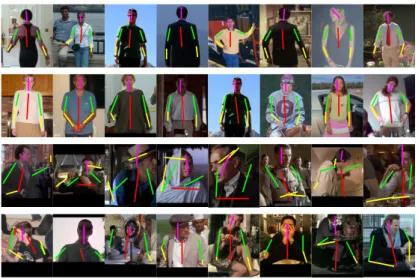
Our pose evaluator successfully detects cases where the HPE algorithms succeed or fail, as shown in figure 9. In general, an HPE algorithm fails where there is self-occlusion or self-occlusion from other objects, when the person is very close to the image borders or at an extreme scale, or when they appear in very cluttered surroundings. These cases are caught by the HPE evaluator.
5
Conclusions
Human pose estimation is a base technology that can form the starting point for other applications, e.g. pose search [10] and action recognition [21]. We have shown that an evaluator algorithm can be developed for human pose estimation methods where no confidence score (only a MAP score) is provided, and that it accurately predicts if the
Fig. 9:Example evaluations.The pose estimates in the first two rows are correctly classified as successes by our pose evaluator. The last two rows are correctly classified as failures. The pose evaluator is learnt using the regime B and with a CPC threshold of0.3. Poses in rows 1,3 are estimated by Eichner and Ferrari [5], and poses in rows 2,4 are estimated by Yang and Ramanan [22].
algorithm has succeeded or not. A clear application of this work is to use evaluator to choose the best result amongst multiple HPE algorithms.
More generally, we have cast self-evaluation as a binary classification problem, us-ing a threshold on the quality evaluator output to determine successes and failures of the HPE algorithm. An alternative approach would be to learn an evaluator by regressing to the quality measure (CPC) of the pose estimate. We could also improve the learning framework using a non-linear SVM.
We believe that our method has wide applicability. It works for any part-based model with minimal adaptation, no matter what the parts and their state space are. We have shown this in the paper, by applying our method to various pose estimators [5, 16, 2, 22] with different parts and state spaces. A similar methodology to the one given here could be used to engineer evaluator algorithms for other human pose estimation methods e.g. using poselets [4], and also for other visual tasks such as object detection (where success can be measured by an overlap score).
Acknowledgments
We are grateful for financial support from the UKIERI, the ERC grant VisRec no. 228180 and the Swiss National Science Foundation.
References
1. G. Aggarwal, S. Biswas, P.J. Flynn, and K.W. Bowyer. Predicting performance of face recog-nition systems: An image characterization approach. InIEEE Conf. on Comp. Vis. and Pat. Rec. workshops. IEEE Press, 2011, pages 52 –59.
2. M. Andriluka, S. Roth, and B. Schiele. Pictorial structures revisited: People detection and articulated pose estimation. InIEEE Conf. on Comp. Vis. and Pat. Rec. IEEE Press, 2009. 3. M. Boshra and B. Bhanu. Predicting performance of object recognition. Pattern Analysis
and Machine Intelligence, IEEE Transactions on, 22(9):956 –969, 2000.
4. L. Bourdev and J. Malik. Poselets: Body part detectors trained using 3d human pose anno-tations. InIEEE Int. Conf. on Comp. Vis. IEEE Press, 2009, pages 1365 –1372.
5. M. Eichner and V. Ferrari. Better appearance models for pictorial structures. In A. Cavallaro, S. Prince, and D. Alexander, editors,Proceedings of the British Machine Vision Conference, pages 3.1–3.11. BMVA Press, 2009.
6. M. Eichner, M. Marin, A. Zisserman, and V. Ferrari. Articulated human pose estimation and search in (almost) unconstrained still images.ETH Technical report, 2010.
7. M. Everingham, L. Van Gool, C. K. I. Williams, J. Winn, and A. Zisserman. The pascal visual object classes (voc) challenge. International Journal of Computer Vision, 88(2), 2010. 8. P. Felzenszwalb, D. McAllester, and D. Ramanan. A discriminatively trained, multiscale,
deformable part model. InIEEE Conf. on Comp. Vis. and Pat. Rec. IEEE Press, 2008. 9. P. F. Felzenszwalb and D. P. Huttenlocher. Pictorial structures for object recognition.
Inter-national Journal of Computer Vision, 61(1):55–79, 2005.
10. V. Ferrari, M. Marin-Jimenez, and A. Zisserman. Pose search: Retrieving people using their pose. InIEEE Conf. on Comp. Vis. and Pat. Rec. IEEE Press, 2009.
11. V. Ferrari, M. Marin-Jimenez, and A. Zisserman. Progressive search space reduction for human pose estimation. InIEEE Conf. on Comp. Vis. and Pat. Rec. IEEE Press, 2008. 12. O. Mac Aodha, G.J. Brostow, and M. Pollefeys. Segmenting video into classes of
algorithm-suitability. InIEEE Conf. on Comp. Vis. and Pat. Rec. IEEE Press, 2010, pages 1054 –1061. 13. L. Pishchulin, A. Jain, M. Andriluka, T. Thormahlen, and B. Schiele. Articulated people detection and pose estimation: Reshaping the future. InIEEE Conf. on Comp. Vis. and Pat. Rec. IEEE Press, 2012, pages 3178 –3185.
14. D. Ramanan. Learning to parse images of articulated bodies. In B. Sch¨olkopf, J. Platt, and T. Hoffman, editors,Advances in Neural Information Processing Systems 19, pages 1129– 1136. MIT Press, Cambridge, MA, 2007.
15. R. Ronfard, C. Schmid, and W. Triggs. Learning to parse pictures of people. In Springer, editor,European Conference on Computer Vision, volume 4, Copenhague, Denmark, 2002. 16. B. Sapp, A. Toshev, and B. Taskar. Cascaded models for articulated pose estimation. In
K. Daniilidis, P. Maragos, and N. Paragios, editors,Computer Vision ECCV 2010, volume 6312 ofLecture Notes in Computer Science, pages 406–420. Springer Berlin Heidelberg, 2010.
17. W.J. Scheirer, A. Bendale, and T.E. Boult. Predicting biometric facial recognition failure with similarity surfaces and support vector machines. InIEEE Conf. on Comp. Vis. and Pat. Rec. workshops. IEEE Press, 2008, pages 1 –8.
18. P. Viola and M. J. Jones. Robust real-time face detection.International Journal of Computer Vision, 57(2):137–154, May 2004.
19. Peng Wang, Qiang Ji, and J.L. Wayman. Modeling and predicting face recognition system performance based on analysis of similarity scores. Pattern Analysis and Machine Intelli-gence, IEEE Transactions on, 29(4):665 –670, april 2007.
20. Rong Wang and B. Bhanu. Learning models for predicting recognition performance. In IEEE Int. Conf. on Comp. Vis. IEEE Press, 2005., volume 2, pages 1613 –1618 Vol. 2. 21. G. Willems, J. H. Becker, T. Tuytelaars, and L. Van Gool. Exemplar-based action recognition
in video. In A. Cavallaro, S. Prince, and D. Alexander, editors,Proceedings of the British Machine Vision Conference, pages 90.1–90.11. BMVA Press, 2009.
22. Yi Yang and D. Ramanan. Articulated pose estimation with flexible mixtures-of-parts. In IEEE Conf. on Comp. Vis. and Pat. Rec. IEEE Press, 2011.