TECHNICAL UNIVERSITY OF CLUJ-NAPOCA
ACTA TECHNICA NAPOCENSIS
Series: Applied Mathematics, Mechanics, and Engineering Vol. 61, Issue II, June, 2018
KINEMATIC CONTROL FUNCTIONS FOR A SERIAL ROBOT
STRUCTURE BASED ON THE TIME DERIVATIVE JACOBIAN MATRIX
Claudiu SCHONSTEINAbstract: Thekinematic modeling of a mechanical system with n degrees of freedom, involves an impressive volume of computational or differential calculus. There are algorithms dedicated to this task developed in the literature. Applying of algorithms allows a detailed, numerical and / or graphical analysis of kinematics for a mechanical structure, regardless of its type and complexity. The results obtained with algorithms are essential in optimal design, dimensional and energetically, but also to simulate the kinematical and dynamic behavior of the mechanical structures of the robots.
Equation Chapter 1 Section 1
Key words: robotics, time derivative Jacobian Matrix, algorithm, control functions. 1. INTRODUCTION
The kinematics control for a serial robot, is an important task. According to dedicated literature, there are multiple methods to establish the expressions that modeling the kinematic behavior for any mechanical structure. The paper presents a method for kinematic control, based on matrix exponentials, which are the basis for establishing the time derivative for the Jacobian matrix. Hence in the first part of paper, will be presented the mathematical considerations in regarding the obtaining of first derivative for Jacobian matrix. In the second part will be determined the time derivative of the Jacobian matrix, in the case of a serial robot. The third part, presents the kinematic control functions determined on the basis of the time derivative of the Jacobian matrix for the serial structure.
2. THE TIME DERIVATIVE FOR THE JACOBIAN MATRIX
According to the definition expression of the Jacobian matrix [1]-[3], based on the linear and
angular transfer matrix for velocity and accelerations, the time derivative of the Jacobian matrix is defined as: [2]
( )
( )
( )
( )
0 0
6
0 0
; 1
; 1
i i
xn
T
T T
iv i
J J i n
J J i n
q
q W q
é ù
=êë = =úû
éé ù ù
=êêë úû = ú
ê ú
ë û
(1)
where0Jiv
( )
q represents the linear component and0JiW( )
q is the angular component. To establish the time derivative for the Jacobian matrix, according to matrix exponential algorithm from the direct kinematics, the symbolic expression of each column from (1) is:{ } { } { } { }
0
1 2 3 4
i i i i i
J =M J ⋅M J ⋅M J ⋅M J (2) The four matriceal expressions from (2), can be included in a single matrix form as follows:
{ }
i1{ }
i1 { }i1 { }i1M J = êéëME J ME J ME J ùúû (3)
{ }
{ } [ ] [ ]
[ ]
{ }
[ ][ ] [ ] { }
2
2 2
2
0 0
0 0
0 0
i
i i
i
ME J
M J ME J
ME J
é ù
ê ú
ê ú
= ê ú
ê ú
ê ú
ë û
{ }
{ } [ ] [ ]
[ ]
{ }
[ ][ ] [ ] { }
3
3 3
3
0 0
0 0
0 0
i
i i
i
ME J
M J ME J
ME J
é ù
ê ú
ê ú
= ê ú
ê ú
ê ú
ë û
(5)
{ }
( ) ( )
{
( )}
( ) ( )
* 4
0 0 0
0 0
*
, :
;
; 0 ;
0 ; 0 0 .
T
i iv iv iv
T T T
T T
iv i k i i
T T
T T T
iv i k
T T
T T T
iv k
M J M M M where
M v b k i n p k
M v b k i n p
M b k i n
w w w
w
w
w
é ù
= êë úû
é é ù ù
ê ú
=ê êë = úû ⋅D ú
ë û
é é ù ù
=êê êë = úû úú
ë û
é é ù ù
ê ú
=ê ê = ú ú
ë û
ë û
(6)
where i j k m, , ,
1;if i R
; 0; if i T
, is an operator which highlights the type of joint.The time derivative of the expressions (3)- (5), are determined as:
{ }
[ ]{ }
1 [ ]{ }
1
1
0 0
i i
i
ME V ME J
ME V
é ù
ê ú
= ê ú
ê ú
ë û
, (7)
( )
{ }
( )
{ }
1 0 1
3 3 exp 0
i
i j j j
j
d
ME V k x q
dt
-´ =
ì ì üü
ï ï ïï
ï ï ïï
= íï íïå D ýýïï
ï ïî ïïþ
î þ
(8)
( )
{ }
{ }
[ ][ ]
2 2
6 9
3
0 0
i i
x
ME V ME J
I
é ù
ê ú
= ê ú
ê ú
ë û
(9),
where
( )
{ }
( )
{ }
02 3 3 6x i i i
ME V = D ⋅éêI k x ùú
ë û
(10)
{ }
{ }
[ ][ ]
3 3
3
0 0
i i
ME V ME J
I
é ù
ê ú
= ê ú
ê ú
ë û
,
{ }
[ ][ ] [ ]
( )
{ }
[ ]( )
{ }
3 1 2 3 3
1
1 0 2
1
3 0
1
,
: ;
0 0
; exp
0
. exp
i
k
m m m m
m i
n
k k
k k
ME V A A A I
and A
A d k x q
dt k i n
A d
k x q dt
d
=
-=
= é ù ê ú = ê ú ê ú ë û
é ù
ê ú
ê ì üú
ì ü
ê ú
=ê ïïï ïï D ïïïïïú
í í ýý
ê ï ï = ïïú
ï ï ïï
ê ïî î þïþú
ë û
é ù
ê ú
ê ì üú
=êê ïï ìïï üïïïïúú D
í í ýý
ê ïï ïï ïïïïú
ê î î þþú
ë û
å
å
(11)
The time derivative of the column vector bk, from (6), according to [1], [3] is determined as:
( )
( )
{ }
( )( )
{ }
( ) ( )0 3 3 1
2
0 0
sin
1 cos
k k k k
k k k
k k
b l k q
k q v q
´
= + ´ ⋅ ⋅D +
é ù
+ ´ ⋅ -ë ⋅D ⋅û ⋅
(12)
The previous expressions will be applied
(i= 1 n), resulting each column of the time
derivative for the Jacobian matrix as :
( )
{ }
{ } { }{ } { }
{ }
{ } { } { }1 2 3
0
1 2 3
1
1 2 3
,
:
i i i
i i i i iv
i n
i i i
iv iv iv iv
ME J ME J ME J J Trace ME J ME J ME J ME
ME J ME J ME J where ME M w M w M w
=
*
ìé ù ü
ï ⋅ ⋅ ï
ïê ú ï
ï ï
ïê ú ï
ïê ú ï
= íïê ⋅ ⋅ ú⋅ ýï
ïê ú ï
ï ⋅ ⋅ ï
ïê ú ï
ïë û ï
î þ
é ù
= êë úû
(13)
According to literature, the previous expression can be written in a simplified form as results:
( )
{ }
{ } { }{ } { }
{ }
{ } { } { }1 2 3
0
1 2 3
1
1 2 3
i i i iv
i i i i iv
i n
i i i iv
ME J ME J ME J M J ME J ME J ME J M
ME J ME J ME J M w
w
w
* =
é ⋅ ⋅ + +ù
ê ú
ê ú
ê ú
= +ê ⋅ ⋅ + +ú
ê + ⋅ ⋅ ⋅ ú
ê ú
ë û
(14)
As an important remark, the previous obtained Jacobian matrix, contains on one hand the Coriolis terms and complementary themes, and on the other hand the terms referring to centripetal accelerations.
3. DETERMINING THE TIME
DERIVATIVE OF JACOBIAN MATRIX FOR THE SERIAL ROBOT 2TR
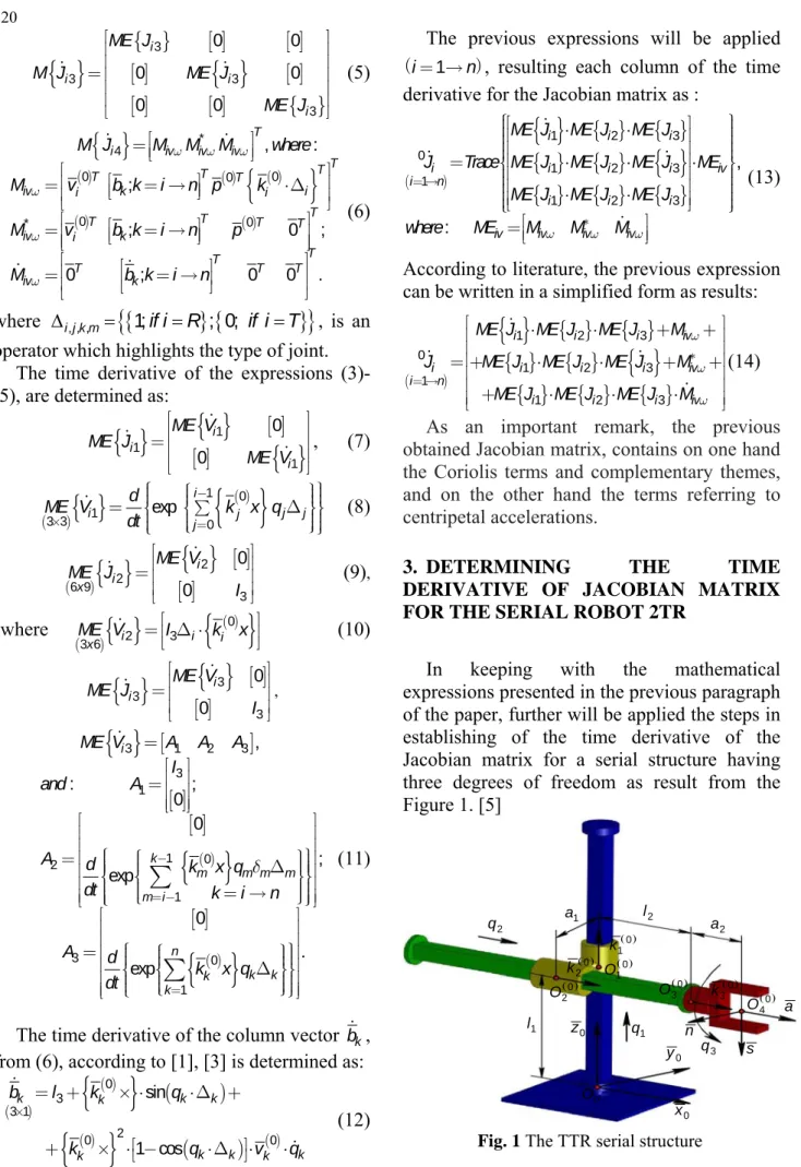
In keeping with the mathematical expressions presented in the previous paragraph of the paper, further will be applied the steps in establishing of the time derivative of the Jacobian matrix for a serial structure having three degrees of freedom as result from the Figure 1. [5]
1
l
1
a
0
O
0 4
O
2
q
1
q
3
q
a s n
0
z
0
x
0
y
2
l
2
a
0 2
O
0 1
O
0 3
O
0 1
k
0 2
k
0 3
k
Hence, there is opened an external loop for
(i= 1 3), and on the basis of (8) results:
{ }
11 [ ]03ME V = (15)
( )
{ }
( ){ }
0{
{ }
( )0}
[ ]21 1 1 1 1 1 3
3 3x exp 0
ME V =éêê k x q⋅ ⋅D ⋅ k x q⋅ ùúú=
ë û
(16)
( )
{ }
( ){ }
0{
{ }
( )0}
[ ]31 2 2 2 2 2 3
3 3x exp 0
ME V =éê k x q⋅ ⋅D ⋅ k x q⋅ ùú=
ê ú
ë û
(17)
In keeping with (15)-(17), introduced in (7), there are obtained the matrices [5],[6], [7]:
{ }
( ){ }
[ ] [ ]{ }
[ ] 1 11 6 1 6 6 0 0 ; 0 i i ME V ME J ME V ´ é ù ê ú=ê ú=
ê ú
ë û
(18)
{ }
( ){ }
[ ] [ ]{ }
[ ] 21 21 6 21 6 6 0 0 ; 0 ME V ME J ME V ´ é ù ê ú=ê ú=
ê ú
ë û
(19)
{ }
( ){ }
[ ] [ ]{ }
[ ] 31 31 6 31 6 6 0 0 . 0 ME V ME J ME V ´ é ù ê ú=ê ú=
ê ú
ë û
(20)
According to (6) and (12), for (i= 1 3)there
are established the following expressions:
( ) ( ) ( ) [ ] ( ) ( ) ( ) [ ] ( ) 0 0
1 1 3
0 1
2
1 2 3 1 3 1 3
1 1 3 1 3
0 0
2 1 1 1
3 1
; 1 3 0 , :
0 0 1 ;
0 0
0 0 1
0 1
T T
T T T
v k
T
T T
T T
T T T
T
M v b k p where
v
q
b b b l sq a cq q a sq l cq
p l a l k w
* =éê é = ù ùú
ê ú ë û ê ú ë û = ì ü
ï é ù é ù é ù ï
ï ï
ï ê ú ê ú ê ú ï
ï ê ú ê ú ê ú ï
ï ï
ï = = = ⋅ + ⋅ - ï
í ê ú ê ú ê ú ý
ï ê ú ê ú ê ú ï
ï ï
ï ê ú ê ú ê ⋅ - - ú ï
ï ë û ë û ë û ï
ï ï
ï ï
î þ
= - D ⋅ [ ]03
T T
é = ù
ê ú ë û (21) ( ) ( ) ( ) [ ] ( ) ( ) ( ) [ ] [ ] w
* =éê é = ù ùú =
ê ú ë û ê ú ë û ìïï = ïï ïï
ïìï é ù üï
ïï é ù ï
ïï ê ú ê ú ï
ïï ï
ïï ê ú ê ú ï
ïï - ï
=ííïï =ê ú = ⋅ê + ⋅ ú ýï
ê ú
ê ú
ïï ï
ïï ê ú ê ⋅ - ⋅ - ú ï
ïï ë û ë û ï
ïïïî ïïþ
ïï
ï é ù
ïï ê = - ú
ë û
î
0 0
2 2 3
0 2
2
3 2 3 1 3 1
3 1 3 1
0
2 1 1 3 3
; 2 3 0
10 0 0 1 0 1 0 0 T T
T T T
v k T T T T T T T T
M v b k p
v
q
cq b b l sq a
cq a sq l
p l a l
üïï ïï ïï ïï ïï ïï ýï ïï ïï ïï ïï ï ï ï ï ïþ (22) ( ) ( ) ( ) [ ] ( ) ( ) ( ) [ ] [ ] w
* =éê é = ù ùú =
ê ú ë û ê ú ë û ì ü ï ï
ï = ï
ï ï
ï ï
ï ï
ï ï
ï ìï é ù üï ï
ï ï ï ï
ï ï ê ú ï ï
ï ï ï ï
ï ï ê ú ï ï
ï ï = ⋅ + ⋅ - ï ï
í í ê ú ý ý
ï ï ê ú ï ï
ï ï ï ï
ï ï ê ⋅ - ⋅ - ú ï ï
ï ï ë û ï ï
ï ïïî ïïþ ï
ï ï
ï ï
ïé ù
ïïê = - ú
ïë û
ïî þ
0 0
3 3 3
0
1 1 3
3 3 1 3 1
3 1 3 1
0
2 1 1 3
3
; 3 0
0 0 1 1 0 T T
T T T
v k T T T T T T
M v b k p
v l a
cq b l sq a
cq a sq l
p l a l ïïïï ï (23) [ ] [ ] [ ] [ ] ( ) ( ) [ ] 1
3 1 3 1 3 1
3 1
2
1 3 1 3
1 2 3 3
1 3 1 3
1 3
6 1
; 1 3
0 0 0
0 0 0 0 0 0 0 T T
T T T
v k
x x x
T x T T T T
T T T
T
x
M b k
q
a sq l cq
b b b q
a cq l sq
q q
w
é é ù ù
ê ú
=ê ê = ú ú =
ë û
ë û
ìïï ïï
ïïìï üï
é ù
é ù é ù
ï ï
ï ê ú ê ú ê ú ï
ï ê ú ê ú ê ú ï
ï ï
ï ⋅ - ⋅ ï
=ííï =ê ú =ê ú = -ê ⋅ ú ýï
ê ú
ê ú ê ú
ï ï
ï ê ú ê ú ê ⋅ + ⋅ ⋅ ú ï
ï ë û ë û ë û ï
ï ï ï ï î þ üïï ïï ïï ï ï ï ï ï ï ï ï ï ï ï ïý ï ï ï ï ï ï ï ï ï ï ï ï ï ï ï ï ï ï ï ï ï ï ï ï î þ (24) [ ] [ ] [ ] [ ] ( ) ( ) [ ] 2
3 1 3 1 3 1
3 1
2
1 3 1 3
1 2 3 3
1 3 1 3 3
3 1
; 2 3
0 0 0
0 0 0 0 0 0 0 0 T T
T T T
v k
x x x
T x
T T
T T
T T T
T x
M b k
q
a sq l cq
b b q b
a cq l sq q
w
é é ù ù
ê ú
=ê ê = ú ú =
ë û
ë û
ìïï ïï ïï
ïìï é ù üï
ïïï é ùê ú ê ú é ùê ú ïï
ï ê ú ê ú ê ú ï
ï ï
ï ⋅ - ⋅ ï
=ííï =ê ú = -êê ⋅ úú =ê ú ýï
ê ú ê ú
ï ï
ï ê ú ê ⋅ + ⋅ ⋅ ú ê ú ï
ï ë û ë û ë û ï
ï ï ï ï î þ üïï ïï ïï ïï ï ï ï ï ï ï ï ïý ï ï ï ï ï ï ï ï ï ï ï ï ï ï ï ï ï ï ï ï ï ï ï ï î þ (25) [ ] [ ] [ ] [ ] ( ) ( ) [ ] 3
3 1 3 1 3 1
3 1
1 3 1 3
3 3
1 3 1 3 3
6 1
; 3
0 0 0
0
0
0
T T
T T T
v k
x x x
T x T T T T x
M b k
a sq l cq
b q
a cq l sq q w
é é ù ù
ê ú
=ê ê = ú ú =
ë û ë û ì ü ï ï ï ï ï ï ï ï ï ï ï ï
ïìï é ù üï ï
ïï ï ï
ïï ê ú ï ï
ïï ï ï
ïï ê ú ï ï
ïï ⋅ - ⋅ ï ï
=ííïï = -ê ⋅ ú ý ýï ï
ê ú
ïï ï ï
ïï ê ⋅ + ⋅ ⋅ ú ï ï
ïï ë û ï ï
ïïïî ï ïïþ
According to previous expressions, the time derivative for the Jacobian matrix in the case of the serial structure from Figure 1, becomes:
{ }
{ } { }{ } { }
{ }
{ } { } { }[ ]
11 12 13 1
0
1 11 12 13 1
6 1
11 12 13 1
0
v v
x v
ME J ME J ME J M J ME J ME J ME J M
ME J ME J ME J M w
w
w
*
ì ü
ï ⋅ ⋅ ⋅ +ï
ï ï
ï ï
ï ï
ï ï
= +íï ⋅ ⋅ ⋅ + =ýï
ï ï
ï+ ⋅ ⋅ ⋅ ï
ï ï
ï ï
î þ
(27)
{ }
{ } { }{ } { }
{ }
{ } { } { }
[ ]
21 22 23 2
0
2 21 22 23 2
6 1
21 22 23 2
0
v v
x v
ME J ME J ME J M J ME J ME J ME J M
ME J ME J ME J M w
w
w
*
ì ü
ï ⋅ ⋅ ⋅ +ï
ï ï
ï ï
ï ï
ï ï
= +íï ⋅ ⋅ ⋅ + =ýï
ï ï
ï + ⋅ ⋅ ⋅ ï
ï ï
ï ï
î þ
(28)
{ }
{ } { }{ } { }
{ }
{ } { } { }[ ]
31 32 33 3
0
3 31 32 33 3
6 1
31 32 33 3
0
v v
x v
ME J ME J ME J M J ME J ME J ME J M
ME J ME J ME J M w
w
w
*
ì ü
ï ⋅ ⋅ ⋅ + ï
ï ï
ï ï
ï ï
ï ï
= +íï ⋅ ⋅ + + =ýï
ï ï
ï + ⋅ ⋅ ⋅ ï
ï ï
ï ï
î þ
(29)
Substituting (27)-(29) in definition expression (1), there is obtained [5],[6] :
( )
[ ]0
6 30x
J q = (30) The time derivative, for the Jacobian matrix in the case of the structure TTR. According to (30), duet o the fact that is a simple mechanical structure, the time derivative is null.
4 DIRECT KINEMATICAL MODELING FOR 2TR SERIAL ROBOT
According to [1], [2], [3] to establish the operational kinematical parameters, for any serial robot structure, there is needed the Jacobian and it time derivative, which are substituted in the following generalized expression:
[ ]
( )
( )
( )
w q q
q q q
w
éé ù ù é ù
é ù êê ú ú ê ú é ù
ê ú ëê û ú ê ú ê ú
ê ú ê ú =ê ú⋅ê ú
ê ú ê ú ê ú ê ú
ê ú ê ú ê ú ê ú
ê ú éê ù ú ê úë û
ë û êëêë úû úû ë û
0 0 0
0
0 0
0 0 0
0
... ... ... ....
T
T T
n n
T
T T
n n
v J
X =
J J X v
(31)
representing the expressions of the column vector of operational velocities and accelerations, which form the direct kinematics equations, with respect to fixed reference frame.
In the case of the mechanical structure, presented in the Figure 1, the expression(31), becomes:
[ ]
( )
( )
( )
w q q
q q q
w
éé ù ù é ù
é ù êê ú ú ê ú é ù
ê ú ëê û ú ê ú ê ú
ê ú ê ú =ê ú⋅ê ú
ê ú ê ú ê ú ê ú
ê ú ê ú ê ú ê ú
ê ú éê ù ú ê úë û
ë û êëêë úû úû ë û
0 0 0
0 3 3
0 0
0 0 0
3 3
0
... ... ... ....
T
T T
T
T T
v J
X =
J J X v
(32)
where, the Jacobian matrix, according to [5], and [6] is:
( )
( )
q
´
é ù
ê ú
ê ú
ê ú
ê ú
ê ú
ê ú
ê ú
é ù
=êë úû= ê ú
ê ú
ê ú
ê ú
ê ú
ê ú
ê ú
ê ú
ë û
0 0 0 0 1 2 3 6 3
0 1 0 0 0 0 1 0 0 .... .... ....
0 0 1 0 0 0 0 0 0
J J J J (33)
The direct kinematics equations, with respect to fixed reference frame { }0 , are
obtained on the basis of (33) and (30), which substituted in (32), are leading to:
( )
q q wé ù é ù
ê ú ê ú
ê ú é ù ê ú
ê ú ê ú ê ú
é ù ê ú ê ú ê ú
ê ú ê ú ê ú ê ú
ê ú ê ú ê ú ê ú
ºê ú= ⋅ =ê ú⋅ê ú=ê ú
ê ú ê ú ê ú ê ú
ê ú ê ú ê ú ê ú
ë û ê ú ê ú
ê ú ë û
ê ú ê ú
ê ú ê ú
ê ú ê ú
ë û ë û
2 1 0
3
1
0 0
2 3 0
3
3
0 1 0
0 0 0 0 1 0 0
...
0 0 1
0 0 0 0 0 0 0 0 q q
v q
X J q
q q
; (34)
( )
q q( )
q q wé ù é ù
ê ú ê ú
ê ú é ù ê ú
ê ú ê ú ê ú
é ù ê ú ê ú ê ú
ê ú ê ú ê ú ê ú
ê ú ê ú ê ú ê ú
ºê ú= ⋅ + ⋅ =ê ú⋅ê ú=ê ú
ê ú ê ú ê ú ê ú
ê ú ê ú ê ú ê ú
ë û ê ú ê ú
ê ú ë û
ê ú ê ú
ê ú ê ú
ê ú ê ú
ë û ë û
2 1 0
3
1
0 0 0
2 3 0
3
3
0 1 0
0 0 0 0 1 0 0
...
0 0 1
0 0 0 0 0 0 0 0 q q
v q
X J J q
q
q
(35)
5 THE EQUATIONS OF INVERSE KINEMATIC MODEL BASED ON JACOBIAN MATRICES
Knowing the direct kinematics equations, based on the Jacobian matrices and its time derivative, according to [1],[2], [4], the inverse kinematics equations can be expressed as:
( )
( )
[ ] ( ) [ ]
( ) [ ] ( )
( ) ( ) ( )
0 1
0
0
1 1 0
0 0
0 0
.... ... 0
X t J t
t
X t t J t J t J t
q q
q q q q q
--
-ì ü
ï ï
ì ü
ï ï
é ù ï éê ùú ï ïï ïï
ê ú ïï ë û ïïï ï
ê ú=ïí ï ïý í⋅ï ïïý
ê ú ï ï ï ï
ê ú ïï ï ïï ï ïï
ê ú ï êé úù - éê ùú ï ï êé úù⋅ ï ë û ïî ë û ë û ï ïþ ïî ë û ïïþ
.(36)
where 0Jéêëq( )t ùúû-1 represents the inverse of the Jacobian matrix. According to [8], the kinematic singularities are characterized by the null value of the determinant associated to the Jacobian matrix. Therefore, in order to avoid this possible situation, which blocks the operation of the robot, the kinematical command functions can be determined by applying the pseudoinverse method, based on Greville's Algorithm, developed in [9], [10]. The inverse kinematic model according to [1], is established having as starting expression (36) , which is leading to the following:
( )
( ) ( )
( )
( )
( )
( )
( )
( )
( )
( )
0 0
1
0 0
1 1
0 0 0 0
;
;
. X t J t t
t J t X t
t J t X t J t J t
q q
q q
q q q q q
--
-é ù
= êë úû⋅
é ù
= êë úû ⋅
é ù é ù é ù
= ëê úû ⋅ - ëê ûú ⋅ êë úû⋅
; (37)
On the previous considerations, in the case of 2TR serial structure, in keeping (33), the inverse of the Jacobian matrix is;
-é ù
ê ú
ê ú
= ê ú
ê ú
ê ú
ë û
1
0 0 1 0 0 0 1 0 0 0 0 0 0 0 0 1 0 0
J (38)
Substituting the previous expression in (37), there is obtained:
( ) ( ) ( )
( )
( )
1
0 0
2 1 3
1 2 3
0 0 1 0 0 0
1 0 0 0 0 0 0 0 0 0 0 0 1 0 0
T
T
t J t X t
q q q
q q q
q = éêëq ùúû- ⋅ =
é ù
ê ú
ê ú
=ê ú⋅ =
ê ú
ê ú
ë û
=
(39)
1 1
0 0 0 0
2 1 3
1 2 3
0 0 1 0 0 0
1 0 0 0 0 0 0 0 0 0 0 0 1 0 0
T
T
t J t X t J t J t
q q q
q q q
(40)
which are expressing the kinematic control functions of the 2TR type serial structure.
6. CONCLUSION
The paper, is dedicated to revealing of the inverse kinematical model, known also as kinematic control functions for a serial robot. Having as starting point the matrix exponential functions, on the basis of Jacobian matrix, there have been determined the first time derivative, for the velocity transfer matrices.
7. REFERENCES
[1] I., Negrean, Mecanică Avansată în Robotică, Editura UT PRESS, Cluj-Napoca, 2008, ISBN 978-973-662-420-9.
[2] Negrean, I., Schonstein, C., Kacso, K., Duca, A., Matrix Exponentials and Differential Principles in the Dynamics of
Robots, The 13-th World Congress in
Mechanism and Machine Science, Guanajuato, Mexico, 19-25 June, 2011.
[3] Negrean, I., Schonstein, C., Advanced Studies on Matrix Exponentials in Robotics, Published in the Acta Technica Napocensis, Series: Applied Mathematics and Mechanics, Nr. 53, Vol. I, 2010, pp. 13-18, Cluj-Napoca, ISSN 1221-5857, Romania.
[4] Negrean, I., Matrix Modelling Formalism in Robot Kinematics, The 6th International Conference on Applied Mathematics and Mechanics, Cluj-Napoca, Acta Technica Napocensis, Series: Applied Mathematics and Mechanics, 1998.
[5] Schonstein, C., Contribuții în dezvoltarea unei structuri robotizate hibride, PhD Thesis, Cluj-Napoca, 2011.
[6] Schonstein, C., Establishing the Jacobian matrix for a three degrees of freedom serial structure, Published in the Acta Technica
Napocensis, Series: Applied Mathematics and Mechanics, Nr. 61, Vol. I, 2018, Cluj-Napoca, ISSN 1221-5872, Romania.
[7] Schonstein, C., Negrean, I., Panc N., - Geometrical modeling using matrix exponential functions for a serial robot
structure, published in Acta Technica
Napocensis, Series: Applied Mathematics, Mechanics and Engineering, Vol. 60, Issue III, 2017, ISSN 1221-5872, Cluj-Napoca, Romania.
[8] Negrean, I., Negrean, D. C., The Matrix-Differentiating Operators in Robot
Kinematics, Cluj-Napoca, October 2001,
Acta Technica Napocensis, Series: Applied Mathematics and Mechanics, 2001, Vol. 2. [9] Chang, R.J., Jiang, T.C., Dynamic Model
and Response of Robot [8]Manipulators with Joint Irregularities, In: ASME Journal of Dynamic Systems, Measurements and Control, Vol. 115, March 1993, pp.70-76. [10] Negrean, I., Negrean, D. C., Matrix
Exponentials to Robot Dynamics, International Conference on Automation, Quality and Testing, Robotics, AQTR 2002, Cluj-Napoca.
„Funcţiile de control cinematic pentru o structură serială bazate pe derivata în raport cu timpul a matricei Jacobiene”
Pentru modelarea cinematică a unui sistem mecanic cu n grade de libertate, care implică un volum impresionant de calcule fie matriceale fie diferenţiale, în literatura de specialitate există dezvoltaţi o serie de algoritmi dedicaţi acestui domeniu. Aplicarea algoritmilor, permite o analiză detaliată, sub formă numericăşi/sau grafică, cu privire la cinematica structurii analizate, indiferent de tipul şi complexitatea acesteia. Rezultatele obţinute cu ajutorul algoritmilor, sunt esenţiale în proiectarea optimală, sub aspect dimensional şi energetic, dar şi pentru simularea comportamentului cinematic şi dinamic al structurilor mecanice din componenţa roboţilor.