Document Image Analysis by Probabilistic Network and
Circuit Diagram Extraction
András Barta and István Vajk
Department of Automation and Applied Informatics Budapest University of Technology and Economics H-1111, Budapest, Goldmann Gy. tér 3., Hungary E-mail: [email protected]
Keywords: Document processing, Bayesian network, Object recognition Received: December 15, 2004
The paper presents a hierarchical object recognition system for document processing. It is based on a spatial tree structure representation and Bayesian framework. The image components are built up from lower level image components stored in a library. The tree representations of the objects are assembled from these components. A probabilistic framework is used in order to get robust behaviour. The method is able to convert general circuit diagrams to their components and store them in a hierarchical data-structure. The paper presents simulation for extracting the components of sample circuit diagrams. Povzetek: Predstavljen je sistem za prepoznavanje objektov pri obdelavi dokumentov.
1 Introduction
Optical technology has gone through significant development during the past few years. Still enormous quantities of documents are in printed form, making them difficult to store and access. Automatic document processing should be able to provide a solution. The documents should be digitalized, their information extracted and stored in a format that retains this structured information. Several good solutions exist for document processing and analysis, but their efforts are mainly focused on character registration tasks. This paper tries to find a solution for a special document processing application, interpreting circuit diagrams. Many old blue-prints of electrical equipment are sitting on shelves. Converting them to a meaningful digital representation would make it possible to search and retrieve them by content.
In this paper we present a method to convert general circuit diagrams to their components and store them in a hierarchical data-structure. The task of an object recognition system is to represent images by a set of image bases. In this research a hierarchical structure of bases is selected in order to be able to represent the complexities of the circuits.
Circuit reconstruction has to be performed at several levels. At the lowest level the image pixels are processed and low level image objects, edges, lines and arcs are extracted. At the middle level the basic circuit components are constructed from these elements. At the highest level the electrical connections of the components are interpreted. This paper deals mainly with the middle part. Many papers investigate low level image processing algorithms; for example Heath [19] provides a good comparison of the most frequently used edge detecting methods. Rosin [21] investigates ellipsis fitting
and also compares some of the methods. Arc extraction is also well treated in the literature [24]. At the high end the electrical interpretation is highly application dependent and it is not treated here.
In image processing the selection of data structure is important and open question. Generally the structural relationships of the object components can be captured by graphs [7]. In many vision applications, however, simpler data structure is sufficient to represent the image components. In this research tree structure is used. Tree structures are widely applied for image processing tasks. In many cases the object recognition is treated as a tree isomorphism problem [13], [14]. In tree isomorphism the tree of the object is created and compared against a library tree. In our research a different approach is used: the tree is identified by an adaptive process and only those image components are processed that are necessary for growing the tree.
lack the hierarchical object representation capabilities. In the next section the related literature is overviewed in more detail. The extracted information consists of two components the library that contains the image bases and the coding of the input circuit diagram. In order to be able to encode images the system has to go through a two phase learning process. First the image bases of the library and then the network parameters are learned. In section 3 a few issues related to image coding are investigated. Section 4 treats the theoretical background that is used for creating the document processing system. Bayesian network, network parameter learning and the visual vocabulary creation is investigated here. Section 5 shows how network inference can be implemented for circuit diagram extraction. It also presents a simulation for extracting the components of sample circuit diagrams. Section 6 explores the possibility of using the presented method for integrated document processing. Finally the last section concludes the paper by raising some issues to extend the method for other applications.
2 Related Work
Document image processing generally is performed at several levels. The first step is separating the input image into coherent areas of image types. The typical image types are text, drawing and picture. The second step is extracting the low level image elements. For drawing interpretation that means vectorization of the image to lines, circles, curves, and bars. At the third step the image components are interpreted and grouped together to form higher level objects.
Page layout segmentation is well treated in the literature. Haralick [33] provides a survey of the early page segmentation methods. These works are mainly bottom-up or top-down algorithms. O'Gorman [3] presents page layout analysis based on bottom-up, nearest-neighbour clustering of page components. Nagy et al. [35] use a top-down approach that combines structural segmentation and functional labelling. Horizontal and vertical projection profiles are used to split the document into successively smaller rectangular blocks. Neural networks [36] can also be used for separating the different areas of an image.
Several methods were suggested for extracting the basic drawing elements. The thinning-based methods [37] use some iterative erosion approach to peel off boundary pixels until a one-pixel wide skeleton is left. The skeleton pixels are then connected by line segments to form point chains. The disadvantage of the method is that line thickness information is lost. Pixel tracking methods [32] track line area by adding new pixels. For vectorization any low level image processing algorithm can be used [19], [21], however they do not provide a general framework for processing all kinds of drawing elements. Deformable models are also frequently used tools for line detection. Song [31] suggests an integrated system for segmentation and modelling in his OOPSV (Object-Oriented Progressive - Simplification - Based Vectorization System) system. General curves can be detected also by optimization. Genetic optimization is
used in [40]. This work also provides an overview of the different curve detecting methods.
Part based structural description has a long history. Several systems have been created for general object recognition that used structural information to represent objects: VISION (Hanson, Riseman, 1978), SIGMA (Hwang at al., 1986) , SPAM (McKeon at al., 1985), ACRONYM (Brooks, Binford, 1981), SCHEMA (Draper et al., 1989). These systems, their successes and failures are investigated by Draper [34]. He writes, "knowledge-directed vision systems typically failed for two reasons. The first is that the low- and mid-level vision procedures that were relied upon to perform the basic tasks of vision were too immature at the time to support the ambitious interpretation goals of these systems. The other impediment was that the control problem for vision procedures was never properly addressed as an independent problem ".
Okazaki at al. proposes a method for processing VLSI-CAD data input [38]. It is implemented for digital circuitry where the components are mainly loop-structured symbols. Symbol identification is achieved by a hybrid method, which uses heuristics to mediate between template matching and feature extraction. The entire symbol recognition process is carried out under a decision-tree control strategy. Siddiqi at al. present a Bayesian inference for part based representation [40]. The object subcomponents are represented by fourth order polynomials. The recognition is based on geometric invariants, but it does not provide a data-structure for representing the components. A similar approach to our research was taken by Cho and Kim [41]. They modelled strokes and their relationships for on-line handwriting recognition. Their system also used Bayesian networks for inference, but only for fixed models. They also assumed Gaussian distributions which can not be applied for circuit diagram analysis.
3 Image Representation
An image is modelled by a set of ξi image bases
(
)
( ) i i( )
i
I x =
∑
h ξ x . (1) The selection of hi functions determines the model type.argues that this increase can be explained and modelled by an overcomplete basis set and sparse coding [26],[27]. In a sparse coding representation only a few bases are used to represent a given image, the contribution of the others are set to zero. In computerized image processing systems at the lowest level the image is represented by pixel bases. This representation is highly redundant. Some redundancy is needed to achieve robust representation in case where the image is corrupted with noise. In this work we try to select an overcomplete basis set. Olshausen's work considers only a flat structure; the image bases are localized wavelet type structures. In this research hierarchical structures of bases are used, thus sparsness and overcompleteness has slightly different interpretation. Not only the horizontal but the vertical distributions of the bases are important. We investigate this in a little more detail in section 5.
4 Network Representation
Bayesian networks are well suited for image processing applications because they can handle incomplete knowledge. Bayes network is used for our research because of the following advantages:
- provides probabilistic representation - provides a hierarchical data structure - provides an inference algorithm
- separates the operating code from the data representation
- it is capable of processing both predictive ad diagnostic evidence
- provides and inhibiting mechanism that decreases the probabilities of the not used image bases Bayesian network representation definition includes the following steps:
1. Selecting the data representation for the nodes. The data representation can be continuous or discrete. In the latter case the definition of the number of possible states is necessary.
2. Encoding the dependences with the conditional probabilities p y x( | ). This applies a x→y network connection, where x y, are two nodes of the network. This dependency quantifies the casual relationships of the nodes and also defines the network connections.
3. Constructing a prior probability distribution,
( )
p x . This distribution describes the background knowledge.
Based on the network definition various inference problems can be solved. The main advantage of the Bayesian framework is that both predictive and diagnostic evidence can be included. The predictive evidence e+ provides high level hypothesis support and it propagates downward in the network. The diagnostic evidence e− is the actually observed event and it provides an upward information flow. This message propagation can be applied to casual polytrees or singly connected networks that is networks with no loops. This
bidirectional flow provides the inference of the network. It can be calculated by the Pearl's message passing algorithm [8]. The predictive and diagnostic evidence is separated and the propagation of their effect is described by two variables, the λ and π messages,
( ) ( | )
( ) ( | )
x p x
x p x
λ π
= =
-+
e
e . (2)
The probability of the node given the evidence is calculated from these messages based on the Bayes rule.
( | , ) ( | , ) ( | )
( | ) ( | ) ( ) ( )
p x p x p x
p x p x x x
α
α αλ π
=
= =
+ - - + +
- +
e e e e e
e e , (3)
where αis a normalizing constant. The propagation from one node to the other is controlled by the conditional probability p y x( | ). In case of trees the messages are calculated by the following propagation rules:
( ) ( )
j
Y j
x x
λ =
∏
λ (4)( ) ( | ) X( )
u
x p x u u
π =
∑
π( ) ( ) ( | )
X x
u x p x u
λ =
∑
λ .( ) ( ) ( )
j k
Y Y
k j
x x x
π απ λ
≠
=
∏
A node receives messages from all of its child nodes and sends a message to its parent (Figure 1).
X
Y Z
U
( )
X u
λ
( )
X u
π
( )
Z u
λ
( )
Z x
π
( )
Y x
λ
( )
Y x
π
Figure 1: Message passing
This local updating can be performed recursively. Every node has a probability value that quantifies the belief of the corresponding object. The objects with high belief values are identified as the real objects of the image.
4.1 Node Description
How to assign the physical meaning to the nodes is a crucial issue. Here, we define the node value to identify the image bases. If the library contains L bases or image features, then the nodes can take the value of 1,2,..,L. The model also introduces a belief or probability value at each node. This value determines the probability that the given image feature describes the image based on the evidence or knowledge. The value of the node has multinomial probability distribution with L-1 possible states
1 2 1
( , ,..., K | )
p l l l − e ,
where li is the library reference or index to the ξiimage
image. This provides a robust description, since it is not necessary to achieve exact match for the identification.
Since objects are position dependent, their description should be position dependent also. That means that to describe an object by image bases they have to be transferred to the position of the object. In this work the image base transformation includes displacement, rotation and scaling. The objects have hierarchical structure. Every feature or image element is described by the combination of other transferred image elements. In other words, an image feature is represented by lower level image bases
1
( ( ), ) n
j i i i
i
T
ξ ξ
=
=
∑
a r , (5)T is an operator that performs an orthogonal linear transformation on the image bases. The parameters of the transformation are stored in the riparameter vector. The
image bases may be parameterized by an aiattribute
vector. Since features belong to parameterized feature classes the ai vector is necessary to identify their
parameters. This description defines a tree structure. The tree is constructed from its nodes and a library. The library is a list of common, frequently used image bases. Figure 2 illustrates the object tree and the library.
3 1 2 2 4 2 1 Library trees Object tree 2 4 3 2 1 1 3
1 1 2
Figure 2: Example tree representation
Visual information is inherently spatially ordered, so the tree is defined to represent these spatial relationships. This transformation has three components, displacement, rotation and scaling. The four parameters of the transformation of node i are placed in a reference vector
r r r
i = ⎣⎡ i si ϕi⎤⎦
r x , (6)
where xir= ⎣⎡xir yir⎤⎦ is the position of the image
element in the coordinate system of its parent node, siris
the scaling parameter and r i
ϕ is the rotation angle. With the object tree, the object library and the image coordinate system the object can be reconstructed. A picture element or a feature is represented in its own local coordinate system. Since only two-dimensional objects are used therefore the scale factor is the same for both axes. Each image base is defined in a unit coordinate system and stored in the library. When the image of an object is reconstructed the image base is transformed from the library to a new coordinate system, which can be described by the vector; ii=
[
xi si ϕi]
.This coordinate system is calculated from the ri
reference vector of the node and the image coordinate
system of the parent node, ii−1. This is a recursive
reconstruction that iterates through the tree.
1 1 1 1 1 1 1 1 cos sin sin cos i i r
i i i i
i i
r
i i i
r
i i i
s
s s s
ϕ ϕ
ϕ ϕ
ϕ ϕ ϕ
− − − − − − − − ⎡ ⎤ = + ⎢ ⎥ − ⎣ ⎦ = = +
x x x
(7)
With this reconstruction algorithm the tree representation of an object can be compared against the image.
4.2 Network Parameters
The network structure is determined by the p y x( | )
conditional probabilities, where x y, are nodes of the network. Conditionally independent nodes are not connected by edge. In order to define the network the
( | )
p y x parameters have to be calculated. These parameters can be assessed based on experimental training data. In our case of document processing the network is trained on circuit diagrams. Here, it is assumed that the image bases of an object description are independent. The probability parametersθi j, are learned
as relative frequencies. It can be shown that the distribution of the θi j, parameters is a Dirichlet
distribution [22], [4]. The conditional probabilities of the network can be described by
1 1 2 1 1
1 2 1 1 2
1 ( )
( , ,..., ) ...
( )
L
N N N
L L K
k k
n p
n
θ θ θ θ −θ − θ −
− = Γ = = Γ
∏
1 2 1 1 2
( , ,..., L ; , ,..., L)
Dirθ θ θ − n n n
= (8)
where nk is the number of time node k occurs in the
sample data and
1 L k k n n =
=
∑
is the sample size. The Γ( )x function for integer values is the factorial function,( )x (x 1)!
Γ = − . The parameters of the Dirichlet distribution correspond to the physical probabilities and the relative frequencies,
( i| i) i
p x=l θ =θ (9)
( ) i
i n
p x l
n
= =
The other important feature of the Dirichlet distribution is that it can be easily updated in case of new data,
1 2 1
1 2 1 1 1 2 2
( , ,..., | )
( , ,..., ; , ,..., )
K
L L L
Dir
Dir n m n m n m
θ θ θ θ θ θ
−
−
=
= + + +
d
and the probability of the data is
1 ( ) ( ) ( ) ( ) ( ) L k k k k n m n p
n m = n
Γ + Γ
=
Γ +
∏
Γd (10)
the calculation is much more complicated. In that case the application of approximating methods is necessary [5]. The ( )p x prior probability is estimated also from the data.
4.3 Creating Visual Vocabulary
The image or document is described by the visual vocabulary. The visual vocabulary consists of a hierarchical structure of image bases. The creation of the image bases is a fundamental part of the image processing system. The image base library can be created several ways: created by human input, learned by a supervised method and created by an automatic process. We have researched all of the methods.
4.3.1 Manual Coding
With a good user interface manual object definition can be a helpful tool, especially in the early stages of the library development process. In this research low level image processing is not performed, therefore the most basic building blocks such as lines, circles, arcs are programmed directly into the code. In a general object recognition system these features should be the results of a lower level image processing algorithms.
4.3.2 Supervised Learning
The image bases can be acquired by human supervision by the following way. The image of a base is created. The object recognition algorithm identifies those components of the image, which are already in the library. The spatial relationships of these components are calculated and the object tree is created. This tree with additional user supplied information can be placed into the library. By performing this process sequentially more and more complex objects can be taught. If a square, for example, is learned as a tree of four lines, then it can be used as a new image base for further processing. This way the library can be created by a sequence of images. Similar approach is used by Agarwal, Awan and Roth for creating vocabulary of parts for general object recognition task [28].
4.3.3 Unsupervised Learning
The library objects can be also learned by an automatic process. In this method the objects are identified as the repetitive patterns of the image. During the learning process a histogram of random groups of image components is created. The most frequently occurring configurations are identified as objects and placed in the library. These library objects can be used as image bases in a new recognition step.
The image base selection can be improved by the application of Gestalt theory, which says that the main process of our visual perception is grouping [15]. Objects with similar characteristics get grouped and form a new higher level object, a Gestalt. Such characteristics are proximity, alignment, parallelism and connectedness.
The Helmholtz principle quantifies this theory [29]. It states that objects are grouped if the number of occurrences is higher than it would be in a random arrangement. As we investigated in section 3 the number and the overcompleteness of the basis set is also important.
The calculation of the structural complexity of the different representations helps control the basis set selection process. If the number of bases is increased, the representation is simpler, but the complexity representing the object library will be higher. The structural complexity quantifies how complex the objects are. It is an important quantity, because during the object recognition from the complex pixel representation a simplified object representation is gained. Generally the representation of an object by image elements is not unique. In order to evaluate the many different representations a distance measure definition is necessary which quantifies the internal complexity of the objects. The structural complexity of an object is the shortest possible description of the structural relationships of the object. The complexity of a tree representation is defined as
( )
( )
1 ( )
n
T o l l
l
c o c c I
=
= T +
∑
T (11) where c T( o) represents the complexity of the object treeand Il is an indicator function. The complexity of an
object consists of the complexity of the object tree and the complexity of the library that is used for the representation. The complexity of a tree is defined as the number of nodes in the tree:
( )
cT = T =n
The structural complexity of the object can be defined as the minimum of the object tree complexity,
(
)
( ) T( )
c o = c o
T
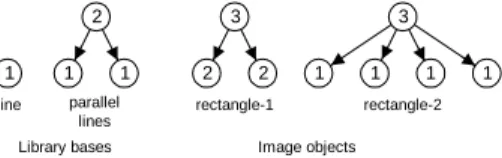
min (12) The minimum is calculated on every possible T tree that represents the object. This is similar to the MDL approach of Rissanen [42]. Generally simpler object description should be preferred against more complex ones. For example a rectangle can be described by several different ways. It can be described by four lines or by two parallel line pair. Figure 3 shows these arrangements
line
1 2
1 1
parallel lines
1 1 1
3 3
2 2 1
rectangle-1 rectangle-2
Library bases Image objects
5. Circuit Diagram Processing
The circuit diagram extraction is carried out for computer generated circuit diagrams. A sample diagram is shown on figure 4. The identification of the image components is performed by calculating the probabilities or beliefs of the corresponding nodes.
Figure 4: A sample circuit drawing
First, the image library is created. The library is created from the circuit diagrams to store the frequently occurring image components. The image library contains the image bases in tree representation along with the conditional probabilities and the rj transformation
parameter vector. A few components from the library which are created from the computer generated circuit diagrams are shown on figure 5.
1 1 1 1 6 1 1 1 5
1 2 3
4
1 1
line circle arc plus triangle rectangle
9 gnd 4 5 1 1 11 1 1 opamp
1 1 1 1 1 1 1 1
8
capacitor
Figure 5: Library tree example
The conditional parameters are calculated from the sample circuit diagrams. The θ parameters of the Dirichlet distribution are the relative frequencies. In a typical Bayesian network the direction of the edge shows the casual relationships. In image processing applications we can not say whether the object is causing the feature or the feature is causing the object; the edges of the tree may go in either direction. The direction depends on whether we are using a generative or descriptive model [25]. Sarkar and Boyer [30] for example in a similar work defined the edges in a reverse (upward) direction. The effect of edge reverser can be calculated by the Bayes rule.
In this research the conditional probabilities are calculated for both directions. Since the algorithm uses upward and downward processing this simplifies the calculations. The upward (x←y) conditional probability can be calculated from the relative frequencies. Based on the definition the conditional probability is
/
( )
( | )
( ) /
x y x y
y y
n n n
p x y p x y
p y n n n
∩ ∩
∩
= = = (13)
where nyis the number of times y occurs and nx∩y is the
joint occurrence of x and y. For example for the operational amplifier,
8
( | ) 0.0755
106
opamp line
line n p opamp line
n ∩
= = =
For the downward (x→y) conditional probability calculation the library object definitions are used. Unity distribution is assumed on each downward edge of the nodes. For example on Figure 5 the edges of the operational amplifier (l=11) have equally 1/6 probability. In order to perform proper network propagation, the Bayes rule should be satisfied. The validity of this unity distribution assumption can be demonstrated by the following calculations. The Bayes rule is
( | ) ( ) ( | )
( )
p x y p y p y x
p x
= (14)
The denominator can be calculated by the law of total probability 1 1 ( ) ( | ) ( ) x x i i i k k
x y y
i i
i i y
n n p x p x y p y
n n
∩
= =
=
∑
=∑
(15)where kx is the number of children of node x and yi are
the child nodes of x.
1 1
( | )
x x i
i
i
x y y
y y
y x y x y x x x
k k y
x y x x x x x
x y
i i
n n
n n n n n k k
p y x
n n k n k k
n n ∩ ∩ ∩ ∩ ∩ = = = = = = =
∑
∑
∑
. i y xk is the number of children of node x with identical library index, for which yi
x x
k =k
∑
. The summation is for different library index child nodes. For example1 triangle opamp
k = , plus 1 opamp
k = , line 4 opamp
k = and the conditional probabilities p plus opamp( | )=1/ 6,
( | ) 1/ 6
p plus opamp = , p line opamp( | )=4 / 6, which is a
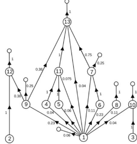
unity distribution over the edges because there are four lines. 6 4 11 1 7 13 8 9 12 10 3 2 5 0.04 0.11 0.23 0.11 0.38 0.075 0.23 0.04 0.06 0.04 1 1 0.75 1 1 1 1 0.38 0.06 0.25 0.25 1 1 1 1
The downward probabilities can be calculated based on the library definition. The upward probabilities are calculated from the sample circuit diagram in the following steps. At the start of the algorithm no probabilities can be calculated, because the joint occurrences of the image bases are unknown. First, an initial distribution is calculated for the library and the circuit diagram is processed. Based on the processed circuit, the correct probabilities are calculated. The algorithm with the initial probabilities does not perform as well as with the correct probabilities, but it is sufficient to train the tree. The resulted structure and probabilities that are calculated from the sample circuit diagram are shown on figure 6. This diagram is slightly misleading since there are no loops in the tree, the multiple connected nodes are different instantiations of an image base. The small circles mark the root nodes. They indicate that the image component is not a subcomponent of a higher level object.
5.1 The Algorithm
The recognition process starts by selecting a new image component. This single node tree is expanded by adding a structure shown on figure 7. By adding more and more nodes the whole image tree is created.
a c
Step-1 Step-4
Ste p-2
S tep
-3
Step-6
S
te
p -5 d
b
Figure 7: The steps of the algorithm
This node expansion is performed in the following steps:
Step 1: A new image component (a) is selected randomly based on the node probability distribution. The selection is performed by the roulette-wheel algorithm. In case of new node the prior probability is used.
Step 2: This new evidence starts the belief propagation of the network. Based on the conditional probabilities several object hypotheses are created (b, upward hypothesis). These object hypotheses are described by library index and coordinate system of a node. The coordinate system of the object hypothesis
pi = ⎣⎡ pi spi ϕpi⎤⎦
i x can be calculated by the following coordinate transformation:
cos sin
sin cos
i
pi r
k
r
pi i k
pi pi
r
pi i k pi
pi pi
s s
s
s
ϕ ϕ ϕ
ϕ ϕ
ϕ ϕ
= = −
⎡ ⎤
= − ⎢ ⎥
−
⎣ ⎦
x x x
, (16)
where ii=
[
xi si ϕi]
is the coordinate system of theimage component and r r r
k = ⎣⎡ k sk ϕk⎤⎦
r x is the
reference vector of child node of the library tree.
Step 3: The object hypothesis with the transformation
vector can be projected back to the image based on (7). This projection creates child hypotheses not only for node c, but all of the child nodes of b (for example d).
Step 4: A search is performed to match this projected
child node hypotheses. If this object hypothesis matches one of the already identified subtrees then they are combined. If no match has been found then a new hypothesys are created (downward hypothesis) for the child node. If the child hypothesis is one of the lowest level image components then it is compared against the image, based on a distance measure. This distance measure can be, for example, the Euclidean distance. It should be defined for every basic image element independently; in our case for lines, circles and arcs. The results of the child node comparisons are converted to probability by an arbitrarily chosen function.
Step 5: The probability of the child modes propagates
upward as new evidence. The upward probabilities are combined to calculate the probability of root b.
Step 6: Only the high probability nodes are processed,
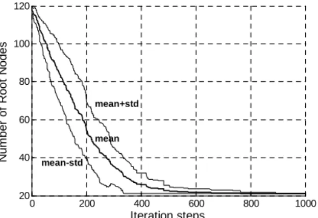
the others are neglected. This is true for both the upward and downward object hypotheses. This process creates a structure with several root nodes. These root nodes can be an input to a next level of recognition step. The root nodes are either subcomponents that the algorithm will grow further or they are the final solutions.
These root nodes are the final solution only for our processing. They can be the input to a higher level processing in which the electrical connections of the circuit diagram are interpreted. Since the number of root nodes quantifies the state of the circuit diagram processing, it can be used to evaluate the performance of the method. The search method is adaptive and local; only certain area of the image is processed at a time. This is advantageous for images with noise or clutter.
0 200 400 600 800 1000
20 40 60 80 100 120
Iteration steps
N
u
m
b
er
of
R
o
o
t N
o
de
s
mean+std
mean-std mean
Figure 8: Evaluation of the algorithm, by the number of root nodes during the recognition
5.2 Complexity of the Algorithm
For a general Bayesian network the worst case computational complexity is n l(2 2+ +2l lkm), where n is
the number of nodes and l is the number of possible states of the nodes and km is the maximum number of
children [22]. The complexity calculation in our case is different, since it is necessary to calculate also the r
spatial transformation parameter vector for every node. The algorithm proceeds by creating upward and downward object hypotheses. The processing of the circuit diagram involves identifying the circuit components as projected library bases. This identification is performed by projections and comparisons; therefore it is unavoidable of having a minimum overhead of calculations. The algorithm is evaluated by the overhead complexity which is calculated from the complexities of the failed and successful object hypotheses. The average wasted calculation of creating one upward (xi←y)
hypothesis is
(
)
0(
)
1
( ) 1 ( | ) ( | )
i
L
u u y
F y H i x i
i
c y µ c p x y k I p x y
=
=
∑
− (17)The algorithmic complexity of calculating one upward hypothesis is u
H
c . This value is constant for every node and it is the sum of the complexity of calculating the spatial transformation and the probability updating.
i
y x k
is the number of the child nodes of node xiwith the same
library index as y. For example if y is a line and xi is an
opamp thenkopampline =4; that is they can be connected four
different ways. The µyterm is added to account for the
symmetries of the objects. I0
(
p x( i| )y)
is an indicatorfunction; its value is 0 if p x( i| )y =0 and 1 otherwise. The complexity, due to the sparse coding does not depend on the library size. It depends only onLuy, the
number of nonzero upward conditional probability values of node y. The right hypothesis is found with p x( i| )y probability therefore the wasted effort is proportional to
1−p x( i| )y . The calculation for every hypothesis propagates downward. The algorithmic complexity of calculating the downward hypothesis for one node is cHd .
This value is constant for every node and it is the sum of the complexity of calculating the spatial projection, the image base comparison and the probability updating. During the downward propagation the projected library base is compared against an image element. In case of failed hypotheses the result of the comparisons are large error term which causes the downward calculations to abort. The numbers of these failed node comparisons are different for every object, but for the complexity estimation an average σ value is used (its typical value is 2-3). The average wasted complexity of a failed object hypothesis is
(
)
0(
)
1
( ) 1 ( | ) ( | )
i
L
d u y
F H y H i x i
i
c y σ µc c p x y k I p x y
=
=
∑
− . (18)In case of successful hypothesis all of the predecessor nodes of the hypothesis tree will be identified, therefore it takes an average n/λn0successful node hypotheses to
identify the full circuit diagram, where n0is the average
object size (number of nodes). The λ constant is necessary because the calculation not always starts at the lowest level nodes; some of the sub-objects are already identified. Its value is between 0 and 1 (it can be set to 0.5). With the above defined values the average complexity overhead can be estimated by
0 ( )
o F
n
c y c
n
λ
= . (19)
The cF value can be calculated by averaging the cF( )y
values for the tree (for worst case analysis maximum can also be used). This is only an approximation of the actual complexity, but it can be used to describe the dependencies of the parameters. The following dependencies can be given for the algorithm:
- The complexity is linear with the number of nodes.
- The complexity does not depend on the size of the library but only on the number of nonzero upward conditional probability values. The complexity is lower if these probability values are concentrated in few high probability entries. - The complexity is lower if the average object size
is higher.
- The complexity is higher if the objects have symmetries.
- The complexity is higher if a node has several child nodes with identical library index (kxyi).
The overall complexity can be reduced by reducing the
i
y x
k values.
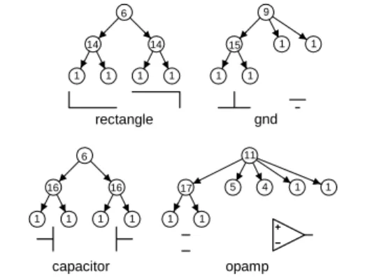
By introducing new image basis for the number of identical children per node can be decreased. Figure 9 shows the expanded trees of a few image bases defined in the previous section.
6
capacitor
1 1
16 16
1 1
4 5
11
1 1
opamp 1 17
1
9
gnd 1
1
1
15 1
6
rectangle
1 1
14 14
1 1
Figure 9: The number identical children per node is reduced by new vertical layer
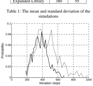
mean and the standard deviation are also calculated. Figure 10 and table 1 show the results.
Mean Std
Original Library 461 149 Expanded Library 380 95 Table 1: The mean and standard deviation of the
simulations
0 200 400 600 800 1000
0 0.02 0.04 0.06 0.08 0.1
Iteration steps
Pr
ob
ab
ili
ty
Figure 10: The histogram of the simulation Original library: dotted curve Expanded library: continuous curve
The simulation clearly shows the complexity is reduced with the new expanded library. That is what we meant in section 2 when we argued about horizontal and vertical overcompleteness.
6 Integrated Document Processing
and Object Recognition
In practical document analysis applications the documents contain different types of image areas: texts, drawings and pictures. Figure 10 shows a sample image with different types of documents. The presented method can be extended to other types of document processing tasks also.
Figure 10: Sample document for integrated processing For character and fingerprint recognition the process can be performed the same way with different library definitions. The same theoretical background can also be applied for general object recognition tasks, but the algorithm needs some modifications. The images of the tools should be segmented. The individual subcomponents should be separated, coded and placed in the library (figure 11). The local and adaptive nature of
the algorithm makes it possible that only a certain portion of the image has to be investigated at a time and it is not necessary to build up the whole image tree.
Figure 11: Image representation by components The presented algorithm can be applied for integrated document processing in two ways. First, a new S node can be defined to select among the different processing steps. The state of the new node will determine which processing task is activated. The state S can be calculated by examining the statistical properties of the image areas. The image areas are marked for the different S values. From the state of node S the probabilities can be recalculated for the individual processing tasks. Figure 12 shows this configuration.
Circuit diagram processing
2
Printed character processing
Hand written character processing
Fingerprint recognition
1 3 4
S I
Image statistics
Figure 12: Integrated document processing The second approach would use one large integrated library. The document image is processed in a unified way and only the image component would determine which image bases are used for the identification. Since the complexity of the presented method does not depend on the library size and the algorithm performs local image processing, this would not carry any additional burden.
hypotheses calculation early, the complexity of the algorithm can be reduced significantly. The performance of the algorithm can be improved further by incorporating more object specific features. For example, for circuit diagram processing the examination of the connectedness of lines would describe the objects better, thus speeding the algorithm up. In this research we intentionally tried to avoid putting any object specific or heuristic knowledge into the algorithm. In the examinations of failed vision systems Draper [34] argues that adding new features for new object classes solves many problems initially but as the system grows they make the system intractable. We considered only such library bases that can be learned by an automatic process. This approach has the significant advantage that the system can be extended to other classes of object recognition. The method is easily expandable to lower level image processing tasks by adding new library elements. Since the algorithm, due to the sparse coding, does not depend on the library size, adding new object description would not increase the complexity.
The presented system performs well, still improvement can be added. The symmetries of the image bases and their effects on the algorithm should be explored more deeply. Lower level image base definitions should be added. Wavelet type image bases are good candidates because they are flexible and they can be easily integrated in library based system. With the low level image bases more testing can be done on real images.
Acknowledgement
The work was supported by the fund of the Hungarian Academy of Sciences for control research and partly by the OTKA fund T042741. The supports are kindly acknowledged.
References
[1] Adams N.J., “Dynamic Trees: A Hierarchical Probabilistic Approach to Image Modelling,” PhD thesis, Division of Informatics, Univ. of Edinburgh
[2] Baum L.E., Petrie, T., Statistical inference for probabilistic functions of finite state Markov chains, Ann.
Math. Statist. 37, pp. 1554–1563, 1966
[3] O'Gorman L., The document spectrum for page layout analysis, IEEE Trans. Pattern Analysis and Machine
Intelligence, 15, November, pp. 1162-1173, 1993
[4] Heckerman D., Bayesian networks for knowledge Discovery, Advances in Knowledge discovery and data
mining, AAAI Press / MIT Press, pp. 273-307, 1996
[5] Chicekering D. M., Heckerman D., Efficient Approximations for the Marginal Likelihood of Bayesian Networks with Hidden Variables, Microsoft Research,
Technical paper MSR-TR-96-08, 1997
[6] Ibañez, M.V., Simó A., Parameter estimation in Markov random field image modeling with imperfect
observations, A comparative study. Pattern recognition
letters 24, pp 2377-2389, 2003
[7] Jolion J.M. and Kropatsch W.G., Graph Based Representation in Pattern Recognition, Springer-Verlag, 1998
[8] Kindermann, R., Snell, J.L., Markov random fields and their application, American Mathematical Society, Providence, RI, 1980
[9] Messmer, B.T., Bunke, H., A decision tree approach to graph and subgraph isomorphism detection, Pattern
Recognition 12, pp. 1979-1998, 1999
[10] Myers, R., Wilson, R.C., Hancock, E.R., Bayesian Graph Edit Distance, Pattern Analysis and Machine Intelligence
6, pp. 628-635, 2000
[11] Pearl, J. Probabilistic Reasoning in Intelligent Systems: Networks of Plausible Interference, Morgan Kauffmann Publishers, 1988
[12] Smyth P., Belief networks, hidden Markov models, and Markov random field: A unifying view, Pattern
recognition letters 18, pp. 1261-1268, 1997
[13] Lu S.Y., A Tree-Matching Algorithm Based on Node Splitting and Merging, IEEE Trans. Pattern Analysis and
Machine Intelligence, vol. 6, no. 2, March, pp. 249-256,
1984.
[14] Jiang T., Wang L., Zhang K., Alignment of Trees–An Alternative to Tree Edit, M. Crochemore and D. Gusfield, eds., Combinatorial Pattern Matching, Lecture Notes in
Computer Science, 807, pp. 75-86. Springer-Verlag,
1994.
[15] Desolneux A., Moisan L., M J., A grouping Principle and Four Applications, IEEE Trans. Pattern Analysis and
Machine Intelligence Vol. 25, No. 4, April, pp. 508-512,
2003
[16] Storkey A.J., Williams C.K.I., Image Modeling with Position-Encoding Dynamic Trees, IEEE Trans. Pattern
Analysis and Machine Intelligence, Vol. 25, No. 7, July
pp. 859-871, 2003
[17] Rock I., Palmer S., The Legacy of Gestalt Psychology,
Scientific Am., pp. 84-90, 1990
[18] Storvik G., A Bayesian Approach to Dynamic Contours through Stochastic Sampling and Simulated Annealing, IEEE Trans. Pattern Analysis and Machine Intelligence, Vol. 16. October , pp 976-986, 1994
[19] Heath M.D., Sarkar S., Sanocki T., Bowyer K.W., A Robust Visual Method for Assessing the Relative Performance of Edge-Detection Algorithms, IEEE Trans.
Pattern Analysis and Machine Intelligence Vol.19, No.
12, December, pp. 1338-1359, 1997
[20] Beaulieu C, Colonnier M, The number of neurons in the different laminae of the binocular and monocular region of area 17 in the cat. The Journal of Comparative
Neurology, 217, pp 337-344, 1983
[21] Rosin P. L., Fitting Superellipses, IEEE Trans. Pattern
Analysis and Machine Intelligence, Vol. 22, No. 7, July,
[22] Neopolitan R. E., Learning Bayesian networks, Pearson Prentice Hall, 2004
[23] McLachlan G.J, Krishnan T., The EM Algorithm and Extensions, John Wiley & Sons, 1997
[24] Song J., Lyu M.R., Cai S., Effective Multiresolution Arc Segmentation: Algorithms and Performance Evaluation
IEEE Trans. Pattern Analysis and Machine Intelligence,
Vol. 26, No. 11, November, pp 1491-1506, 2004
[25] Zou Song-Chun, Statistical Modeling and Conceptualization of Visual Patterns, IEEE Trans.
Pattern Analysis and Machine Intelligence, Vol. 25, No.
6, June, pp 691-712, 2003
[26] Olshausen B.A., Field D.J., Sparse Coding with Overcomplete Basis Set: A Strategy Employed by V1?
Vision Research Vol. 37, No 23, pp. 3311-3325, 1997
[27] Olshausen B.A., Principles of Image Representation in Visual Cortex, The Visual Neurosciences, June, 2002 [28] Agarwal S., Awan A., Roth D., Learning to Detect
Objects in Images via a Sparse, Part-Based Representation, IEEE Trans. Pattern Analysis and
Machine Intelligence Vol. 26, No. 11, November,
1475-1490, 2004
[29] Wertheimer, M. (1923). Laws of organization in perceptual forms, Translation published in Ellis, W. A source book of Gestalt psychology pp. 71-88. London: Routledge & Kegan Paul., 1938, (available at http:// psy.ed.asu.edu/~classics/Wertheimer/Forms/forms.htm ) [30] Sarkar S., Boyer K.L., Integration Inference, and
Management of Spatial Information Using Bayesian Networks: Perceptual Organization, IEEE Trans. Pattern
Analysis and Machine Intelligence, Vol. 15, No. 3,
March, pp 256-274, 1993
[31] Song J., Su F., Tai C. L., Cai S., An Object-Oriented Progressive-Simplification-Based Vectorization System for Engineering Drawings: Model, Algorithm, and Performance, IEEE Trans. Pattern Analysis and Machine
Intelligence, Vol. 24, No. 8, August 2002
[32] Dori D., Liu W., Sparse Pixel Vectorization: An Algorithm and Its Performance Evaluation, IEEE Trans.
Pattern Analysis and Machine Intelligence, Vol. 21, No.
3, pp. 202-215, March 1999.
[33] Haralick R. M., Document image understanding: geometric and logical layout, Proc. IEEE Comput. Soc. Conf. Computer Vision Pattern Recognition (CVPR ),
385-390, 1994.
[34] Draper B., Hanson H., Riseman E., Knowledge-Directed Vision: Control, Learning and Integration, Proceedings of
the IEEE, 84(11), pp. 1625-1637, 1996 (http://
www.cs.colostate.edu/~draper/publications_journal.html) [35] Nagy G., Seth S., Viswanathan M., A Prototype
document image analysis system for technical journals,
IEEE Comp. Special issue on Document Image Analysis
Systems, pp. 10-22, July 1992.
[36] Jain A. K., Zhong Y., Page Segmentation Using Texture Analysis, Pattern Recognition, Vol. 29, No. 5, pp. 743-770, 1996
[37] Janssen R.D.T. , Vossepoel A.M., Adaptive Vectorization of Line Drawing Images, Computer Vision and Image
Understanding, vol. 65, no. 1, pp. 38-56, 1997.
[38] Okazaki A., Kondo T., Mori K., Tsunekawa S., Kawamoto E., An Automatic Circuit Diagram Reader With Loop-Structure-Based Symbol Recognition , IEEE
Trans. Pattern Analysis and Machine Intelligence, Vol.
10, No. 3, pp. 331-341, May 1988
[39] Chen K. Z., Zhang X. W., Ou Z. Y, Feng X. A., Recognition of digital curves scanned from paper drawings using genetic algorithms, Pattern Recognition
36 pp. 123 – 130, 2003
[40] Siddiqi K., Subrahmonia J., Cooper D., Kimia B.B., Part-Based Bayesian Recognition Using Implicit Polynomial Invariants, Proceedings of the 1995 International
Conference on Image Processing (ICIP), pp. 360-363,
1995
[41] Cho S.J., Kim J.H., Bayesian Network Modeling of Strokes and Their Relationships for On-line Handwriting Recognition, Proceedings of the Sixth International Conference on Document Analysis and Recognition
(ICDAR’01), pp. 86-91, 2001