Open Journal Systems

(1)

ISSN 2061-862X 1 Sándor Kovács, Margit Csipkés: A case study of crop structure modelling and decision risks managing by using a stochastic programming model

Magyar Agrárinformatikai Szövetség

Hungarian Association of Agricultural Informatics

Agrárinformatika Folyóirat. 2010. 1. évfolyam 1. szám Journal of Agricultural Informatics. 2010 Vol. 1, No. 1

A case study of crop structure modelling and decision risks managing by using a

stochastic programming model

Sándor Kovács1, Margit Csipkés2

I N F O

Received 16 March 2010 Accepted 19 May 2010 Available on-line 31 May 2010 Responsible Editor: K. Rajkai

Keywords:

crop structure, risk analysis, Monte-Carlo simulation, stochastic programming, and genetic algorithm

A B S T R A C T

We built up a stochastic linear programming crop structure model. We assume the sale prices as well as the yields of the cultivation sectors as stochastic variables and the variables of cost data calculations as deterministic. A farm operating in the Löszhát in Hajdúság provided the data for resources and cultivation technologies. For searching the optimal risk management variety we performed Monte Carlo simulations by using Risk Optimizer 4.5 software. Values of the goal functions were analyzed by statistically. In terms of the measurement of risks we provide different decision alternatives for the crop structure. Evaluating the results of the simulation runs decision makers could choose from alternatives that most suit their risk attitudes.

1. Introduction

In today’s agriculture presenting new challenges (aspects of protection of environment and nature, biomass energy, sustainable development, etc.) only agricultural producers adaptively accommodating to the environment can remain in competition (Balogh et al., 1999). The main condition of this is the combination of both adaptive and optimizing planning. One of the simplest ways of optimizing crop structure is to apply linear programing methods (Csipkés et al., 2008). The use of LP methods, however, is hindered by the great measure of uncertainty to be seen in cultivation. This is due to a number of reasons, therefore, climate, the changeability of weather, pathogens and parasites decreasing the production result, and changes in the economic environment are all important influencing factors, but the change of human factors may also have a negative or positive effect on efficiency.

When a model has uncertain elements a traditional software (like Solver) fail to generate optimal solutions. „In order to find an optimal solution a "brute-force" approach was employed in the past. This involved running an initial simulation, changing one or more values, rerunning the simulation, and repeating this process until what looked like an optimal solution was found. This is a lengthy process, and it is usually not clear how to change the values from one simulation to the next” (Palisade, 2004). The RISKOptimizer Software can take the uncertainty into account existing in the model and reliable optimal solutions can be generated. The RISKOptimizer uses the Monte-Carlo simulation to deal with the uncertainty. In our research we examined the possibilities of planning the crop structure benefiting of the simulation methodology.

2. Applied methods

2.1. Monte-Carlo simulation

The Monte-Carlo method is a generally accepted method of modelling risks, which studies the probable outcome of an event characterized by any input parameters and described by well-known

1_{Sándor Kovács}

University of Debrecen, 4032 Debrecen, Böszörményi út 138., Hungary [email protected]

2_{Margit Csipkés}

(2)

functions. The essence of the Monte-Carlo technique is, on the basis of probability distribution assigned to some uncertain factors, to randomly select values, which are used in each experiment of the simulation (Russel – Taylor, 1997). Monte-Carlo methods are the statistical evaluations of numerical methods and their characteristics using the modelling of random quantities of mathematical solutions (Szobol, 1981). The method is widely used to simulate the likely outcomes of various events and their probability when input parameters are uncertain. In the model to be analyzed we fix the influencing variables and their possible intervals, their likelihood distribution as well as the connections between the variables. A random number generator develops the distribution values of the variables from the given intervals. In our case the simulation model is a stochastic linear programming model, which seeks to examine the behavior of the original system under different varying conditions and circumstances. This also allows us to compare the profitability of various crops and to evaluate decision alternatives. By increasing the number of runs, the expected value of result variants can be given with arbitrary accuracy as follows (Jorgensen, 2000):

(1)

ψ

=Eπ

{

U(X)

}

=

∫

U(x)

π

(x)dx

where

X

=

{ }

θ

,

φ

is the vector containing

θ

decision parameters and φ state parameters. State parameters are the actual selling prices and yields of crops. The most obvious example for decision rules is decision-making on crop structure. We can decide on the usage of the sowing area for growing different crops. The U() function is the function of profitability (in our study it is the profit contribution3). The

E

_π

()

function is the expected value of U() function in the case of some

π

probability distribution. During modelling, several thousands of calculations are performed by randomly choosing one value out of input parameter values, i.e.

{ }

x

(j) , where x(j) were taken from the distribution of

π

. At the end of the simulation, an expected value is gained for the result variant to be determined, which can be calculated as follows (Jorgensen, 2000; David – Scollnik, 2001):

(2) 1

{

U(x(1)) ... U(x(k))

}

k + +

=

ψ

,

where k is the number of simulation runs.

Besides the many advantages (quick and easy calculations with computer, complex mathematics can be included with no extra difficulty) offered by this technique, it is often criticized as being an approximate technique. „However, any required level of precision can be achieved by simply increasing the number of iterations in a simulation. The limitations are in the number of random numbers that can be produced from a random number generating algorithm and the time a computer needs to generate the iterations. These limitations can be avoided by structuring the model into sections” (Vose, 2006). Monte Carlo technique is often combined with Marcov Chains and its sampling methods to improve the efficiency of the technique (Congdon, 2007).

2.2. Optimization procedure

RISKOptimizer uses genetic algorithms (GA) to generate possible values for the sowing areas of crops. The result of this “simulation optimization” is the combination of values for the sowing areas, which maximizes the mean for the simulation results for the profit contribution. „RISKOptimizer runs a full simulation for each possible trial solution that is generated by the GA-based optimizer. In each iteration step of a trial solution's simulations, probability distribution functions in the spreadsheet are sampled and a new value for the target cell is generated. At the end of a simulation, the result for the trial solution is the mean for the distribution of the target cell, which we wish to maximize. This value is then returned to the optimizer and used by the genetic algorithms to generate new and better trial solutions. For each new trial solution, another simulation is run and another value for the target statistic is generated” (Palisade,2004). In order to model uncertainty we used the probability

(3)

distribution functions in @RISK 4.5 and applied Monte-Carlo simulation for selecting random values from these distributions.

2.3. Stochastic LP model

The general form of the model is as follows:

(3)      

≤ →

≤

x x c

b x A

0

max

In formulae 3 the total capacity vector is denoted with „

b

” and „A” indicates the technological matrix, which consists of the per unit demands (mostly in hour/hundred hectares) taking the crop relation and irrigation, labor and equipment into consideration. The rule for crop rotation assures that all crops could remain competitive, while the rule for irrigation was necessary as coleseed and green peas could produce higher yields under irrigation.

The solution vector „

x

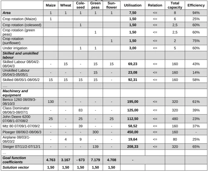
” consists of variables which are the sowing areas of the different crops in hectare. The goal function coefficients are denoted with „c”, they mean per unit incomes or profit contributions. The spreadsheet form of the model can be seen in Table 1.

Table 1. EXCEL Spreadsheet model for determining the optimal crop rotation and managing decision risks

Maize Wheat Cole-seed

Green peas

Sun-flower Utilisation Relation

Total

capacity Efficiency Area 1 1 1 1 1 7,50 <= 8 94%

Crop rotation (Maize) 1 1,50 <= 6 25%

Crop rotation (coleseed) 1 1,50 <= 2,5 60%

Crop rotation (green

peas) 1 1,50 <= 2,5 60%

Crop rotation

(sunflower) 1 1,50 <= 2 75%

Under irrigation 1 1 3,00 <= 5 60%

Skilled and unskilled labour

Skilled Labour

08/04/2-08/04/3 - 15 - 15 15 69,23 <= 160 43%

Unskilled Labour

05/04/3-05/05/1 - - - 15 - 23,08 <= 160 14%

Skilled 08/05/1-08/05/2 15 15 15 15 - 92,31 <= 160 58% ….

Machinery and equipment Berico 1260

08/09/3-08/10/3 130 - - - - 195,00 <= 320 61%

Class Dominator

08/06/3-08/07/1 - - 83 - - 125,00 <= 320 39%

John Deere 6200

07/08/1-07/08/2 25 - 25 - 25 112,50 <= 480 23%

Mtz 80 07/09/1-07/09/2 - - 39 - - 58,52 <= 160 37%

Ploeger 08/06/2-08/06/3 - - - 300 - 450,00 <= 160 -

Airplane

08/03/1-08/03/2 - 4 9 - - 19,64 <= 80 25%

Steiger 07/11/2-07/12/1 - - - 139 - 208,33 <= 320 65% …

Goal function

(4)

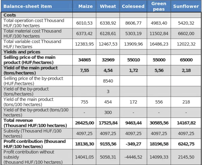
The LP task can be considered stochastic, because the solution vector values come from an uniform distribution on (0,3) interval, while the goal function coefficients (the values of the profit contributions) come from different distributions. In the calculation of their values we take into consideration the actual subsidies as well as the selling prices and yields of the main products, which also come from different distributions (Table 2). The area based subsidy (SAPS) was 2.954,6 Thousand HUF/ hundred hectare in each case, while the additional national subsidy (TOP-UP) was 1.154,1 Thousand HUF / hundred hectare, so the total subsidy was 4.108,7 Thousand HUF / hundred hectare per crop (Table 2).

Table 2. The calculation of Profit Contribution of the different crops in EXCEL

Balance-sheet item Maize Wheat Coleseed Green _peas Sunflower

Costs

Total operation cost Thousand

HUF/100 hectares 6010,53 6338,92 8606,77 4983,40 5420,32 Total material cost Thousand

HUF/100 hectares 6373,42 6128,61 5303,19 11502,84 6602,00 Total variable cost Thousand

HUF/ hectares 12383,95 12467,53 13909,96 16486,23 12022,32

Yields and prices Selling price of the main

product (HUF/hectares) 34865 32969 55010 55000 65000

Yield of the main product

(tons/hectares) 7,55 4,54 1,72 5,56 2,18

Selling price of the by-product

(HUF/hectares) 8540 Yield of the by-product

(tons/hectares) 3 Yield of the main product

(tons/100 hectares) 755 454 172 556 218 Yield of the by-product (tons/100

hectares) - 300 - - -

Total revenue

(Thousand HUF/100 hectares) 26425,00 17525,84 9463,44 30585,56 14167,82

Subsidy (Thousand HUF/100

hectares) 4097,25 4097,25 4097,25 4097,25 4097,25

Profit contribution (thousand

HUF/100 hectares) 18138,30 9155,56 -349,27 18196,58 6242,75

Profit contribution without subsidy

(thousand HUF/100 hectares)

14041,05 5058,31 -4446,52 14099,33 2145,50

Source: own calculation

The goal function values were formed during the simulation runs only if the restrictive conditions are satisfied. Furthermore, we employ another rule, which is that the number of the efficient restrictive conditions must be grater than the number of inefficient conditions. A restrictive condition was inefficient in case the efficiency was below 20 %.

2.4. Data and the applied distributions

In our analysis we have used the data of an agricultural company farming in Löszhát, Hajdúság. The sowing area of the company is 800 hectares the crops grown are winter wheat, maize, winter coleseed, sunflower and green peas. We built into the model the technology used by the company (Table 1).

(5)

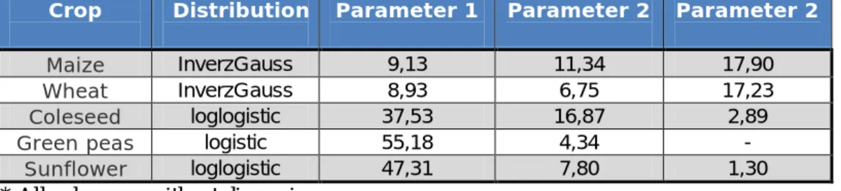
just like the total capacity vector and the per unit demands, may be considered fixed. Within the model, we consider the average yields and the selling prices (the returns from sales) as probability variables. We estimated the distributions and their parameters for modeling both the selling prices and average yields according to the farm data of the Research Institute of Agricultural Economics, North Plains Region for the years 2000-2008 with the help of BestFit 4.5 (Table 3-4).

Table 3. The applied distributions and their parameters for modeling the selling prices*

Crop Distribution Parameter 1 Parameter 2 Parameter 2

Maize InverzGauss 9,13 11,34 17,90

Wheat InverzGauss 8,93 6,75 17,23

Coleseed loglogistic 37,53 16,87 2,89

Green peas logistic 55,18 4,34 -

Sunflower loglogistic 47,31 7,80 1,30

* All values are without dimensions

Table 4. The applieddistributions and their parameters for modeling the average yields*

Crop Distribution Parameter 1 Parameter 2

Maize ExtremeValue 15,25 7,04

Wheat Logistic 17,92 5,62

Coleseed Logistic 44,26 12,07

Green

peas Normal 40,52 17,90

Sunflower Normal 44,08 21,25

* All values are without dimensions

Source: own calculation, based on data provided by the Research Institute of Agricultural Economics

We measure the risk of the Profit contribution with the percentiles of its distribution. On the other hand, production risk of the different crops can be measured by the coefficient of variation.

3. Major research results

The first step in our research was to find an optimal solution for crop structure employing RiskOptimizer and Monte-Carlo simulation. After we have run 5000 simulations, which takes two and a half hours, we gained 118.678 thousand HUF/ hundred hectares for the Profit contribution and a sowing area of 150 hectare for maize, 165,84 hectare for wheat, 12,8 hectare for coleseed, 140,0 for Green peas and 199,18 hectare for sunflower. These values satisfy the rules for crop rotation and areas under irrigation. Subsequent to the optimal solution mainly wheat and maize could be sown regarding profit contribution. The ratio of the area of sunflower is also high. The reason for this is that biodiesel factories will be built in the near future, and the oil from sunflower will have much greater market potentials.

In the second stage of the research we employed a simple Monte-Carlo simulation without optimization in order to manage decision risks. Approximately 50.000 simulation runs were performed by using Risk@ 4.5. Values of the goal function (Figure 1) and the development of the sowing areas were evaluated by scenario analysis (Table 5). Figure 1 shows the percentiles of the Profit contribution calculated by Monte Carlo simulation. Different percentiles indicate different levels of risk and we use them to draw several scenarios.

(6)

at least the given profit contribution. We summarized the results at the given five percentiles (different risk levels) (Table 5).

Figure 1. The percentiles of the Profit contribution

Table 5. Scenarios for the distribution of the sowing area of the crops (in percentage)

Percentile Maize Wheat Coleseed Green peas Sunflower

90% 24,75 19,04 17,36 24,26 14,60

75% 23,63 20,01 18,30 23,25 14,82

50% 22,85 19,99 19,17 22,18 15,81

25% 22,46 20,20 20,10 21,02 16,23

10% 22,24 20,19 20,77 20,41 16,39

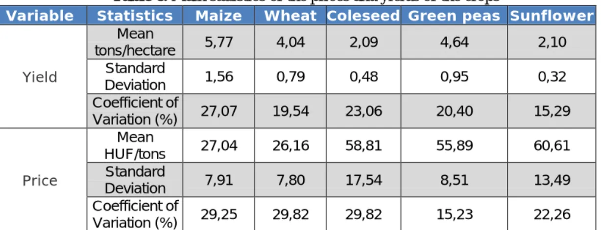
It can be seen from Table 5 that at lower risk levels it is worth increasing the area of wheat, coleseed and sunflower, while taking higher risks (e.g. at the 90th percentile) its worth growing maize and green peas in a much larger area. This conclusion in the case of green peas can be explained by the irrigation technology as well as the higher prices (Table 6), which makes green peas much more competitive. It is obvious from Table 6 that the most risky crops are maize and coleseed, while the less risky crops are green peas and sunflower considering the variation coefficient of yields and prices.

Table 6. Main statistics of the prices and yields of the crops

Variable Statistics Maize Wheat Coleseed Green peas Sunflower

Yield

Mean

tons/hectare 5,77 4,04 2,09 4,64 2,10 Standard

Deviation 1,56 0,79 0,48 0,95 0,32 Coefficient of

Variation (%) 27,07 19,54 23,06 20,40 15,29

Price

Mean

HUF/tons 27,04 26,16 58,81 55,89 60,61 Standard

Deviation 7,91 7,80 17,54 8,51 13,49 Coefficient of

Variation (%) 29,25 29,82 29,82 15,23 22,26

Source: calculated according to the farm data of the Research Institute of Agricultural Economics

According to the decision-makers’ risk taking ability and variation coefficients of the yields and prices the appropriate crop structure could be chosen. What the crop structure concerns we can state

-10000 0 10000 20000 30000 40000 50000 60000

95 90 85 80 75 70 65 60 55 50 45 40 35 30 25 20 15 10 5

Percentiles (%)

P

ro

fi

t c

o

n

tr

ib

u

ti

o

n

(

th

o

u

sa

n

d

H

U

F

(7)

that maize and wheat are of grater importance as these crops constitute a large part in crop structure, The growing of sunflower and green peas might become more important due to the large increase in biodisel production,

4. Conclusions

Traditional planning is still the most often applied method in cultivation, which provides adequate planning, but also determines an increasing shortfall in economic competition, In the midst of new challenges (aspects of the protection of nature and the environment, biomass energy, sustainable development) presented by today’s agriculture, only those agricultural producers can remain in competition who adaptively accommodate to the environment. The condition for that is to achieve a combination of adaptive and optimizing planning, which also has to be methodologically appropriate. In optimizing planning, linear programming models are most often used, however, because of their deterministic nature, in choosing from among decision alternatives, we cannot properly take risk into consideration. Applying simulation models may be a solution, in our work we have presented one such application and also presented the way for implementing stochastic programming models in Risk@ using Monte Carlo simulation. The first step in our researh was to find an optimal solution for crop structure employing RiskOptimizer and Monte-Carlo simulation. We choose wheat, maize, coleseed, green peas and sunflower because these crops are raw materials fro producing biomass. We gained 118.678 thousand HUF/ hundred hectares for the Profit contribution and a sowing area of 150 hectare for maize, 165,84 hectare for wheat, 12,8 hectare for coleseed, 140,0 for Green peas and 199,18 hectare for sunflower. In the second stage of the research we employed a simple Monte-Carlo simulation without optimization in order to manage decision risks. Results of these simulation runs were evaluated by scenario analysis, we drew five scenarios according to the risk level. Our aim was to study the crop structure at different risk levels. At lower risk levels it is worth increasing the area of wheat, coleseed and sunflower, while taking higher risks its worth growing maize and green peas in a much larger area. The most risky crops are maize and coleseed, while the less risky crops are green peas and sunflower considering the variation coefficient of yields and prices. It can also be stated that maize and wheat are of grater importance, as these crops constitute a large part in crop structure.

References

Balogh, P. – A. Bai – L. Posta – F. Búzás. 1999. Analysis of environmental effects of cereals and energy plantations in case of unfavourable agricultural conditions. In Proc. „The resources of the environment and the sustained development”, 15-22, Oradea, Analele Universităţii din Oradea.

Congdon, P. 2007. Bayessian statistical modelling. New York, N.Y.: John Wiley and Sons,5-14.

Csipkés, M. – I. Ertsey – L. Nagy. 2008. Vetésszerkezeti variánsok összehasonlító elemzése a Hajdúságban. In Proc. XI. Nemzetközi Tudományos Napok, 14-21, Gyöngyös, Károly Róbert Főiskola.

David, P - M, Scollnik. 2001. Actuarial modeling with MCMC and BUGS. North American Actuarial Journal. 5(2): 96-124.

Jorgensen, E. 2000. Monte Carlo simulation models: Sampling from the joint distribution of “State of Nature”-parameters. In Proc. Economic modelling of Animal Health and Farm Management, 73-84. Wageningen, Farm Management Group, Department of Social Sciences.

Palisade Ltd. 2004. Risk Optimizer manual, Simulation Optimization for Microsoft Excel. Newfield, N.Y.: Palisade Corporation.

Russel, R. S – B. W, Taylor. 1997. Operations Management, Focusing on quality and competitiveness. New Jersey, Prentice Hall, 610-613.

Szobol, I. M. 1981. A Monte-Carlo módszerek alapjai. Budapest, Műszaki Könyvkiadó, 9-11. Vose, D. 2006. Risk analysis, a quantitative guide. New York, N.Y.: John Wiley and Sons, 17. Wikipedia Encyclopedia. 2010. Definition of Contibution margin,