Using Genetic Algorithms and Dominance Concepts for Generating Reduced Test Data

(1)

Using Genetic Algorithms and Dominance Concepts for Generating

Reduced Test Data

Ahmed S. Ghiduk

Department of Mathematics, Faculty of Science, Beni-Suef University, Egypt E-mail: [email protected]

Moheb R. Girgis

Department of Computer Science, Faculty of Science, Minia University, Egypt E-mail: [email protected]

Keywords:genetic algorithms, software testing, automatic test-data generation, dominance. january

Received:March 6, 2008

Testing takes a considerable amount of the time and resources that are spent on producing software. Testing accounts for approximately 50% of the cost of the development of a software system. Therefore, techniques to reduce the cost of testing would be useful. This paper presents an automatic test-data generation technique that uses a genetic algorithm (GA). This technique applies the concepts of dominance relations between nodes to reduce the cost of software testing. These concepts are used to define a new fitness function to evaluate the generated test data. Finally, the paper presents the results of the experiments that have been conducted to evaluate the effectiveness of the proposed GA technique compared to the random testing (RT) technique. These experiments are used to evaluate the effectiveness of the new fitness function and the technique used to reduce the cost of software testing. Povzetek: Predstavljen je genstski algoritem za zmanjšanje števila testnih podatkov.

1 Introduction

Software testing is the main technique used to improve the quality and increase the reliability of software. Software testing is a complex, labor-intensive, and time consuming task that accounts for approximately 50% of the cost of a software system development [1]. Increasing the degree of automation and the efficiency of software testing can reduce the cost of software design, decrease the time required for software development, and increase the quality of software.

One critical task in the automation of software testing is the automation of the generation of test data to satisfy a given adequacy criterion. Test-data generation is the process of identifying a set of program input data that satisfies a given testing criterion. Test-data generation has two main aspects: test generation technique and application of a test-data adequacy criterion. A test generation technique is an algorithm that generates test data, whereas an adequacy criterion is a predicate that determines whether the testing process is finished.

There has been much previous work in automatically generating test data. Perhaps the most commonly encountered are random test-data generation, symbolic test-data generation, dynamic test-data generation, and recently, test-data generation based on GA.

Random test-data generation consists of generating inputs at random until useful inputs are found (e.g., [2, 3, 4]). The problem with this approach is clear with complex programs or complex adequacy criteria, an adequate test input may have to satisfy very specific

requirements. In such cases, the number of adequate inputs may be quite small compared to the total of inputs, so the probability of selecting an adequate input by chance may be low.

Symbolic test-data generation consists of assigning symbolic values to variables to create an abstract, mathematical characterization of the program’s functionality. With this approach, test-data generation can be reduced to a problem of solving an algebraic expression. Many test-data generation methods that use symbolic execution to find inputs that satisfy a test requirement have been proposed (e.g., [5, 6, 7, 8, 9, 10]). A number of problems are encountered in practice when symbolic execution is used. One of such problems arises in indefinite loops, where the number of iterations depends on a non-constant expression, and the index of array, where data is referenced indirectly. Pointer references also present a problem because of the potential for aliasing.

(2)

programming languages. Second, many systems use gradient descent techniques to perform function minimization and, therefore, they can stall when they encounter local minima.

Several search based test-data generation techniques have been developed (e.g., [13, 14, 15, 16, 17, 18, 19, 20]). These techniques had focused on finding test data to satisfy a number of control-flow and data-flow testing criteria. Genetic algorithms have been the most widely employed search-based optimization technique in software testing [21]. The new features of GAs make them capable of finding the nearly global optimum solution. Test-data generation methods based on genetic algorithms have many problems due to the use of fitness functions that depend on control dependences or branch-distance in its calculations. The fitness function that takes control dependencies into account faces a problem to find an input to traverse a target node within loops. A further problem is the assignment of approximation levels for some classes of program with unstructured control flow. A branch-distance-related problem can occur with nested branch predicates. Once input data is found for one or more of the predicates, the chances of finding input data that also fits subsequent predicates decreases, because a solution for subsequent conditions must be found without violating any of the earlier conditions [22, 23, 24]).

To solve the problem of reducing the cost of software testing, we have developed a new GA-based technique with a new fitness function that reduces the test requirements and overcomes the problems of the previous GA-based test-data generation methods.

This paper presents an automatic test-data generation technique that uses a GA for white-box testing. This technique applies the concepts of dominance relations between nodes to reduce the cost of software testing. These concepts are used to define a new fitness function to evaluate the generated test data.

The paper is organized as follows: Section 2 gives some important definitions. Section 3 describes the proposed technique, which is used to reduce the cost of software testing. Section 4 describes the proposed GA technique for automatic test-data generation, and the results of applying this algorithm to an example program. Section 5 presents the results of the experiments that are conducted to evaluate the effectiveness of the proposed GA compared to the random testing technique, to evaluate the effectiveness of the new fitness function and the technique used to reduce the cost of software testing. Section 6 presents the conclusions and future work.

2 Background

We introduce here some basic concepts that will be used through this work.

2.1 The principles of genetic algorithms

The basic concepts of GAs were developed by Holland [25]. GAs are commonly applied to a variety of problems

involving search and optimization. GAs search methods are rooted in the mechanisms of evolution and natural genetics. GAs draw inspiration from the natural search and selection processes leading to the survival of the fittest individuals. GAs generate a sequence of populations by using a selection mechanism, and use crossover and mutation as search mechanisms [26].

The principle behind GAs is that they create and maintain a population of individuals represented by chromosomes (essentially a character string analogous to the chromosomes appearing in DNA). These chromosomes are typically encoded solutions to a problem. The chromosomes then undergo a process of evolution according to rules of selection, mutation and reproduction. Each individual in the environment (represented by a chromosome) receives a measure of its fitness in the environment. Reproduction selects individuals with high fitness values in the population, and through crossover and mutation of such individuals, a new population is derived in which individuals may be even better fitted to their environment. The process of crossover involves two chromosomes swapping chunks of data (genetic information) and is analogous to the process of sexual reproduction. Mutation introduces slight changes into a small proportion of the population and is representative of an evolutionary step. The structure of a simple GA is given below.

Simple Genetic Algorithm () {

initialize population; evaluate population;

while termination criterion not reached { select solutions for next population; perform crossover and mutation; evaluate population; }

}

The algorithm will iterate until the population has evolved to form a solution to the problem, or until a maximum number of iterations have occurred (suggesting that a solution is not going to be found given the resources available).

2.2 The control flow graph

A program’s structure is conveniently analyzed by means of a directed graph, called control flow graph that gives a graphical representation of the program’s control flow. A directed graph or digraph G= (V, E) consists of a set Vof nodes or vertices, where each node represents a statement, and a set Eof directed edges or arcs, where a directed edge e =(n, m) is an ordered pair of adjacent nodes, called Tailand Headof e, respectively. For a node

(3)

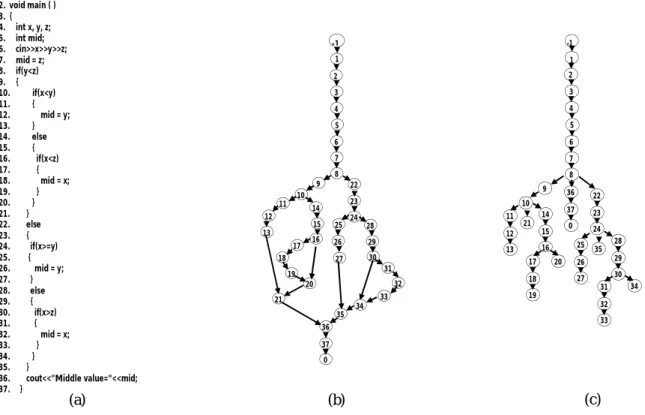
Figure 1: (a) Example program,(b)its Control Flow Graph G,(c) its Dominator Tree DT(G)

(a) (b) (c)

1. #include <iostream.h> 2. void main ( ) 3. { 4. int x, y, z; 5. int mid; 6. cin>>x>>y>>z; 7. mid = z; 8. if(y<z) 9. { 10. if(x<y) 11. { 12. mid = y; 13. } 14. else 15. { 16. if(x<z) 17. { 18. mid = x; 19. } 20. } 21. } 22. else 23. { 24. if(x>=y) 25. { 26. mid = y; 27. } 28. else 29. { 30. if(x>z) 31. { 32. mid = x; 33. } 34. } 35. }

36. cout<<"Middle value="<<mid; 37. }

8 -1

2

3

5

6 1

4

7

36

0 37 11

13 12

17

19 18

14

16 15

31

33 32

28

30 29 22

24 23

35

34 20

9 10

21

25

27 26 9

10 11 12

13 14

15 16 17 18

19 20

21

22

23

24 25

26

27 28

29 30

31 32 33 34 35 36

0 37 8 7 -1

2

3

5

6 1

4

2.3 Dominance

Let G = (V, E)be a digraph with two distinguished nodes

n0and nk. A node ndominates a node mif every path P

from the entry node n0to mcontains n.

Several algorithms are given in the literature to find the dominator nodes in a digraph (e.g., [27] and [28]).

By applying the dominance relations between the nodes of a digraph G, we can obtain a tree (whose nodes represent the digraph nodes) rooted at n0. This tree is

called the dominator tree; we denote it by DT(G). A (rooted) tree DT(G) = (V, E) is a digraph in which one distinguished noden0, called the root, is the Head of no

arcs; every node nexcept the root n0is a Head of just one

arc and there exists a (unique) path (dominance path) from the rootn0to each noden; we denote this path by dom(n). Tree nodes of outdegree zero are called leaves.

For example, Figure1.c shows the dominator tree of the flow graph G (Figure 1.b) of the example program (Figure 1.a). The dominance path of node 21 inDT(G) is

dom(21) = -1, 1, 2, 3, 4, 5, 6, 7, 8, 9, 10, 21.

3 Reducing the cost of testing

This section describes our proposed technique for reducing the cost of software testing that fulfils the all-statements coverage criterion. The proposed technique is based on the concepts of the dominance relations between nodes of the program’s control flow graph. This technique aims to cover a subset of statements (nodes of the program’s control flow graph) that guarantees the coverage of all statements of the tested program.

The set of leaves of the dominator tree is an essential set (i.e., every set of paths that covers it, covers all nodes in the tree). To illustrate the effectiveness of this technique, we apply it to the example program given in Figure 1. The set of leaves of the example program is L = {0, 13, 19, 20, 21, 27, 33, 34, 35}. The dominance paths of the elements of this set are:

dom(0) = -1, 1, 2, 3, 4, 5, 6, 7, 8, 36, 37, 0.

dom(13) = -1, 1, 2, 3, 4, 5, 6, 7, 8, 9, 10, 11, 12, 13.

dom(19) = -1, 1, 2, 3, 4, 5, 6, 7, 8, 9, 10, 14, 15, 16, 17, 18, 19.

dom(20) = -1, 1, 2, 3, 4, 5, 6, 7, 8, 9, 10, 14, 15, 16, 20.

dom(21) = -1, 1, 2, 3, 4, 5, 6, 7, 8, 9, 10, 21.

dom(27) = -1, 1, 2, 3, 4, 5, 6, 7, 8, 22, 23, 24, 25, 26.

dom(33) = -1, 1, 2, 3, 4, 5, 6, 7, 8, 22, 23, 24, 28, 29, 30, 31, 32, 33.

dom(34) = -1, 1, 2, 3, 4, 5, 6, 7, 8, 22, 23, 24, 28, 29, 30, 34.

dom(35) = -1, 1, 2, 3, 4, 5, 6, 7, 8, 22, 23, 24, 35.

Covering an element of the set L guarantees the coverage of its dominance path. It is clear that, the union of nodes of this set of dominance paths is the set of all nodes of the program’s control flow graph (i.e., all statements of the tested program).

(4)

4 GA-based test-data generation

This section describes the proposed GA for automatic test-data generation, which uses a new fitness function to evaluate the generated test data. This new fitness function depends on the concepts of the dominance relations between nodes of the program’s control flow graph. The algorithm searches for test cases that satisfy the all-statements criterion. The major components of this GA are discussed below.

4.1 Representation

The proposed GA uses a binary vector as a chromosome to represent values of the program input variables. The length of the vector depends on the required precision and the domain length for each input variable.

Suppose we wish to generate test cases for a program of kinput variables x1,…, xk where each variable xican

take values from a domain Di= [ai, bi]. Suppose further

that didecimal places are desirable for the values of each

variable xi. To achieve such precision, each domain Di

should be divided into





di

i

a

b





10

equal size ranges. Let us denote by mi the smallest integer such that









10

di



2

mi



1

i

a

b

. Then, a representation

having each variable xicoded as a binary string stringiof

length miclearly satisfies the precision requirement. The

mapping from the binary string stringito a real number xi

from the range [ai, bi] is performed by the following

formula:

1

2 











i

m i i i i i

a

b

x

a

x

(4.1)

Where

x

_i



represents the decimal value of the binary

string stringi[Michalewicz, 1999].

It should be noted that the above method can be applied for representing values of integer input variables by setting dito 0, and using the following formula instead

of formula (4.1):

)

1

2 int(











i

m i i i i

i

a

b

x

a

x

(4.2)

Now, each chromosome (as a test case) is represented

by a binary string of length





k

i i

m

1

; the first m1bits

map into a value from the range [a1, b1] of variable x1, the next group of m2bits map into a value from the range

[a2, b2] of variable x2, and so on; the last group of mkbits

map into a value from the range [ak, bk] of variable xk.

For example, suppose a program has 2 input variables

xand y, where –3.0



x



12.1 and 4.1



y



5.8, and the required precision is four decimal places for each variable. The domain of variable xhas length 15.1; the precision requirement implies that the range [-3.0, 12.1] should be divided into at least 15.1



10000 equal size ranges. This means that 18 bits are required as the first part of the chromosome: 217< 151000



218. The domain of variable y has length 1.7; the precision requirement

implies that the range [4.1, 5.8] should be divided into at least 1.7



10000 equal size ranges. This means that 15 bits are required as the second part of the chromosome: 214< 17000



215. The total length of a chromosome (test case) is then m= 18+15=33 bits; the first 18 bits code x

and remaining 15 bits code y. Let us consider an example chromosome:

010001001011010000111110010100010. By using formula (4.1), the first 18 bits, 010001001011010000, represents x = 1.0524, and the next 15 bits, 111110010100010, represents y= 5.7553. So the given chromosome corresponds to the data values 1.0524 and 5.7553 for the variables xand y, respectively [19].

4.2 Initial population

As mentioned above, each chromosome (as a test case) is represented by a binary string of length m. We randomly generate pop_size m-bit strings to represent the initial population, where pop_size is the population size. The appropriate value of pop_size is experimentally determined. Each chromosome is converted to kdecimal numbers representing values of kinput variables x1,…, xk

(i.e. a test case) by using formula (4.1) or (4.2).

4.3 Evaluation function

The algorithm uses a new evaluation (fitness) function to evaluate the generated test data. This new fitness function depends on the concepts of the dominance relations between nodes of the program’s control flow graph. The algorithm uses this new fitness function to evaluate each test case by executing the program with it as input, and recording the traversed nodes in the program that are covered by this test case. We denote to the set of traversed nodes by exePath. Also, it finds the dominance path dom(n) of the target node n. The fitness function is the ratio of the number of covered nodes of the dominance path of the target node to the total number of nodes of the dominance path of the target node. The fitness value ft(vi) for each chromosome vi (i = 1, …, pop_size) is calculated as follows:

1. Find exePath: the set of the traversed nodes in the program that are covered by a test case.

2. Find dom(n): dominance path of the target node n

(the set of dominator nodes from the entry of the dominator tree to n).

3. Determine



dom

(

n

)



exePath



: uncovered nodes of the dominance path (the difference between the dominance path and the traversed nodes).

4. Determine



dom

(

n

)



exePath





: covered nodes of the dominance path (the complement set of the difference set between the dominance path and the traversed nodes).

5. Calculate



dom

(

n

)



exePath





: number of

(5)

6. Calculate

dom

(

n

)

: number of nodes of the

dominance path of the target node n (cardinality of the dominance set).

Then,





) ( ) ( )

(

n dom

exePath n

dom v

ft _i

 



The fitness value is the only feedback from the problem for the GA. A test case that is represented by the chromosome viis optimal if its fitness value ft(vi)= 1.

4.4 Selection

After computing the fitness of each test case in the current population, the algorithm selects test cases from all the members of the current population that will be parents of the new population. In the selection process, the GA uses the roulette wheel method [29]. This method is described below.

For the selection of a new population with respect to the probability distribution based on fitness values, a roulette wheel with slots sized according to fitness is used. Such roulette wheel is constructed as follows:

 Calculate the fitness value ft(vi) for each

chromosome vi(i = 1,…,pop_size).

 Find the total fitness of the population





pop_ size

i

ft

v

i

F

_

1

(

)

.

 Calculate the relative fitness value rft for each chromosome

F v ft v

rft i

i

) ( )

(  .

 Calculate the cumulative fitness value cft for each chromosome



1 i ) (

pop_size 2,...,

i ) ( ) ( ₁

)

(



i_ _ _

i i

v rft

v rft v cft i

v

cft

.

The selection process is based on spinning the roulette wheel pop_size times; each time we select a single chromosome for a new population in the following way:

 Generate a random (float) number r from the range [0..1].

 If r < cft(v1) then select the first chromosome v1;

otherwise select the i-th chromosome vi(2



i



pop_size) such that

cft

(

v

i

)



r



cft

(

v

i1

)

.

Obviously, some chromosomes would be selected more than once.

4.5 Recombination

In the recombination phase, we use two operators, crossover and mutation, which are the key to the power of GAs. These operators create new individuals from the selected parents to form a new population.

Crossover: It operates at the individual level. During crossover, two parents (chromosomes) exchange substring information (genetic material) at a random position in the chromosome to produce two new strings (offspring). The objective here is to create better population over time by combining material from pairs of (fitter) members from the parent population. Crossover occurs according to a crossover probability.

The probability of crossover PXOVER gives us the expected number PXOVER



pop_size of chromosomes, which undergo the crossover operation. We proceed in the following way:

For each chromosome in the parent population:  Generate a random (float) number r from the

range [0..1];

 If r<PXOVERthen select given chromosome for crossover.

Now we mate selected chromosomes randomly: For each pair of coupled chromosomes we generate a random integer number pos from the range [1..m-1] (m is the number of bits in a chromosome). The number pos

indicates the position of the crossing point. Two chromosomes (b1…bposbpos+1…bm) and

(c1…cposcpos+1…cm) are replaced by a pair of their

offspring (b1…bposcpos+1…cm) and (c1…cposbpos+1…bm). Mutation: It is performed on a bit-by-bit basis. Mutation always operates after the crossover operator, and flips each bit with the pre-determined probability. The probability of mutation PMUTATION, gives us the expected number of mutated bits

PMUTATION



m



pop_size. Every bit (in all chromosomes in the whole population) has an equal chance to undergo mutation (i.e., change from 0 to 1 or vice versa). So we proceed in the following way:

For each chromosome in the current (i.e., after crossover) population and for each bit within the chromosome:

 Generate a random (float) number r from the range [0..1];

 If r< PMUTATIONthen mutate the bit.

In the traditional GA approach the population would evolve until one individual from the whole set which represents the solution is found. In our case, this condition would correspond to finding groups of data items achieving the test requirements (i.e., covering the set of leaves of the dominator tree) of the tested program. We let the population evolves until a combined subset of the population achieves the desired test requirement. The evolution stops when a set of individuals has traversed the dominance path of the test requirement and its fitness value ft(vi)= 1. The solution is this set.

4.6 Elitist

The elitist function enhances the current population by storing the best member of the previous population. If the best member of the current population is worse than the best member of the previous population it exchanges them, and the best member of the current population would replace the worst member of the current population. After that, it stores the best member of the current population.

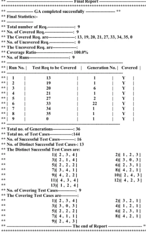
4.7 Example

(6)

contains a table that shows the run number and the test requirement to be covered in this run and the number of the generation in which the test requirement is covered and the status whether it is covered or not. The final statistics shows that we needed 36 generations to obtain 100% coverage of the nine test requirements.

Appendix A shows the part of the result of applying the system to test requirement number 5 (statement 27). This part of the result shows the execution of the steps of the genetic algorithm and operations of our proposed technique.

4.8 Overall algorithm

The proposed GA-based technique accepts as input the program to be tested, the number of input variables, and the domain and precision of each input variable. Also, it accepts the GA parameters: population size, maximum number of generations, and probabilities of the crossover and mutation operators. The algorithm produces a set of test cases, the set of nodes covered by these test cases, and the list of uncovered nodes, if any.

The algorithm selects, one at a time, an uncovered node of the set of leaves nodes of the dominator tree and evolves the initial test data until the required test data are obtained or the maximum number of generations is exceeded. Whenever a node is covered, the test case that caused this coverage is stored in a score board. The technique checks the coverage of remaining uncovered nodes by the generated test data that cover the current node. The overall algorithm is presented in Figure 3.

5 Empirical evaluation

This section presents the results of the experiments that have been carried out to evaluate the effectiveness of the proposed GA compared to the random testing (RT)

technique, and to evaluate the effectiveness of the proposed fitness function. A set of nine C++ programs is used in the experiments. To achieve a fair comparison, the random test-data generator was designed to randomly generate sets of pop_sizetest cases in each iteration. The used GA parameters were as follows: Maximum Number of Generations MAXGENS = 100, PXOVER = 0.8 and

PMUTATION= 0.15.

Table 1 shows the reduction percentage of the test requirements. Column#2 shows the total number of test requirements which are demanded by the all-statements criterion and column#4 gives the number of the reduced test requirements. The reduction percentage is 83.3% for prog# 6 and prog# 9 and 75.6% for prog#2. It is clear that the reduction percentage isn’t less than 75%. These results show the effectiveness of the proposed technique to reduce the cost of all-statements testing by reducing the number of the test requirements.

** --- Final Report ---********************************************************************* ** --- GA completed successfully --- **

** Final Statistics:-**

---** Total number of Req.---: 9 ** No. of Covered Req.---: 9

** The Covered Req. are---: 13, 19, 20, 21, 27, 33, 34, 35, 0 ** No. of Uncovered Req.---: 0

** The Uncovered Req. are---: ** Coverage Ratio---: 100.0% ** No. of Runs---: 9

** ---** | Run No. | Test Req to be Covered | Generation No. | Covered | ** ---** | 1 | 13 | 1 | Y | ** | 2 | 19 | 1 | Y | ** | 3 | 20 | 6 | Y | ** | 4 | 21 | 1 | Y | ** | 5 | 27 | 2 | Y | ** | 6 | 33 | 22 | Y | ** | 7 | 34 | 1 | Y | ** | 8 | 35 | 1 | Y | ** | 9 | 0 | 1 | Y | ** ---** Total no. of Generations---: 36

** Total no. of Test Cases---:144 ** No. of Successful Test Cases---: 16 ** No. of Distinct Successful Test Cases-: 13 ** The Distinct Successful Test Cases are:

** 1)[ 2 , 3 , 4 ] 2)[ 1 , 2 , 3 ] ** 3)[ 2 , 1 , 4 ] 4)[ 3 , 0 , 3 ] ** 5)[ 2 , 2 , 2 ] 6)[ 2 , 3 , 1 ] ** 7)[ 3 , 4 , 1 ] 8)[ 4 , 2 , 1 ] ** 9)[ 4 , 2 , 2 ] 10)[ 2 , 4 , 3 ] ** 11)[ 4 , 3 , 4 ] 12)[ 4 , 2 , 3 ] ** 13)[ 1 , 2 , 4 ]

** No. of Covering Test Cases---: 9 ** The Covering Test Cases are---:

** 1)[ 2 , 3 , 4 ] 2)[ 3 , 2 , 1 ] ** 3)[ 3 , 0 , 3 ] 4)[ 1 , 2 , 1 ] ** 5)[ 2 , 2 , 2 ] 6)[ 2 , 3 , 1 ] ** 7)[ 4 , 1 , 1 ] 8)[ 4 , 2 , 1 ] ** 9)[ 2 , 4 , 3 ]

** --- The end of Report --- ** *******************************************************************

Figure 2: The Final Report.

/* A GA algorithm to automatically generate test cases for a given program */ Input:

The program to be tested P; Number of program input variables; Domain and precision of input data; Population size;

Maximum no. of generations (Max_Gen); Probability of crossover;

Probability of mutation; Output:

Set of test cases for P, and the set of nodes covered by each test case; List of uncovered nodes, if any;

Begin

Step 0: Setup (Analysis P to find prerequisites)

1. Classify the program’s statements. 2. Build the program’s control flow graph CFG. 3. Build the program’s dominator tree DT. 4. Find the set of leaves L of the dominator tree. 5. Instrument P to obtain P'.

Step 1: Initialization

Initialize the score board to zero; nRun ← 0;

Set of test cases for P ← φ;

nCases ← 0;

Step 2: Generate test cases

For each uncovered node and not selected before in the set of nodes to be tested (L) Begin

nRun ← nRun + 1;

Create Initial_Population;

Current_population ← Initial_Population;

No_Of_Generations ← 0;

For each member of current population do Begin

Convert the current chromosome to the corresponding set of decimal values; Execute P' with this data set as input;

Evaluate the current test case; If (the current node is covered) then

Mark the current node as covered; End If

End For;

Keep the best member of the current population;

While (current node is not covered and No_Of_Generations ≤ Max_Gen) do

Begin

Select set of parents of new population from members of current population using roulette wheel method;

Create New_Population using crossover and mutation operators; Current_Population ← New_Population;

For each member of Current_Population do Begin

Convert current chromosome to the corresponding set of decimal values; Execute P' with this data set as input;

Evaluate the current test case; If (the current node is covered) then

Mark the current node as covered; End If

End For;

Elitist function: If the best member of the current population is worse than the best member of the previous population then exchange them, and the best member of the current population would replace the worst member of the current population.

Increment No_Of_Generations; End While;

If (the current node is covered) then nCases ← nCases + 1;

Add this test cases to set of test cases for P; Update the score board;

Check all uncovered nodes by this test case. End If

End For;

Step 3: Produce output

Return set of test cases for P, and set of nodes covered by each test case; Report on uncovered nodes, if any;

End.

(7)

Table 1: The reduction percentage of the cost of software testing

Prog# Program Size ProgSize)

No. Of Variable

No. of Test Requirements

(nTestReq)

Reduction percentage= 100*(1 -nTestReq/ProgSize)% 1 42 3 8 80.9% 2 37 3 9 75.6% 3 27 2 5 81.4% 4 41 2 9 78% 5 38 2 7 81.5% 6 36 2 6 83.3% 7 33 2 7 78.7% 8 19 1 4 78.9% 9 18 2 3 83.3%

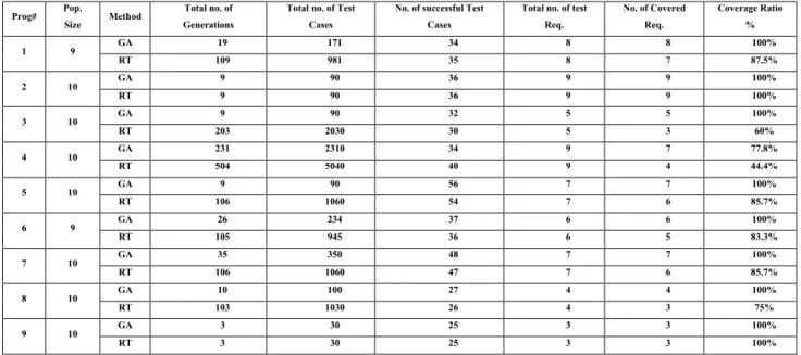
Table 2 shows the results of applying the proposed GA technique and the RT technique to nine C++ programs. These results show the effectiveness of the proposed GA technique over the random testing technique where the GA covers 100% of the set of test requirements in 8 programs while random testing covers 100% of the set of test requirements in 2 programs. In program 3, the GA needed only 9 generations and 90 test cases to reach 100% coverage while RT needed 203 generations and 2030 test cases to reach 60% coverage. In program 4, the GA needed 231 generations and 2310 test cases to reach 77.8% coverage while RT needed 504 generations and 5040 test cases to reach 44.4% coverage.

6 Conclusions and future work

This paper presented an automatic test-data generation technique that uses a genetic algorithm. This technique applies the concepts of dominance relations between nodes to reduce the cost of software testing. These concepts used to define a new fitness function to evaluate the generated test data.

Experiments have been carried out to evaluate the effectiveness of the proposed GA technique compared to the RT technique, and to evaluate the effectiveness of the new fitness function and the technique used to reduce the cost of software testing. The results of these experiments showed that the proposed GA technique outperformed the RT technique in 7 out of the 9 programs used in the experiments. In the other two programs, the proposed GA reached the same coverage percentage as the RT technique. The experiments also showed that the proposed technique reduced the cost of software testing by more than 75%. Also, the results of the experiments showed that the new fitness function is quite suitable to evaluate the generated test-data and showed the usefulness of the concepts of dominance relations between nodes of the program’s control flow graph in reducing the number of test requirements.

This technique is being modified to generate test data for data flow testing. The concepts of dominance relations between nodes of the program’s control flow graph will be used to define a new fitness function to evaluate the generated test data for data flow testing.

Table 2: A comparison between the proposed GA technique and the RT technique.

Prog# Pop.

Size Method

Total no. of Generations

Total no. of Test Cases

No. of successful Test Cases

Total no. of test Req.

No. of Covered Req.

Coverage Ratio % 1 9 GA 19 171 34 8 8 100%

RT 109 981 35 8 7 87.5% 2 10 GA 9 90 36 9 9 100%

RT 9 90 36 9 9 100%

3 10 GA 9 90 32 5 5 100% RT 203 2030 30 5 3 60% 4 10 GA 231 2310 34 9 7 77.8%

RT 504 5040 40 9 4 44.4% 5 10 GA 9 90 56 7 7 100% RT 106 1060 54 7 6 85.7% 6 9 GA 26 234 37 6 6 100% RT 105 945 36 6 5 83.3% 7 10 GA 35 350 48 7 7 100% RT 106 1060 47 7 6 85.7% 8 10 GA 10 100 27 4 4 100% RT 103 1030 26 4 3 75% 9 10 GA 3 30 25 3 3 100%

RT 3 30 25 3 3 100%

References

[1] B. Beizer (1990). Software Testing Techniques. Second Edition, Van Nostrand Reinhold, New York.

[2] H. D. Mills, M. D. Dyer, and R. C. Linger (1987). Cleanroom Software Engineering. IEEE Software 4(5), pp. 19-25.

(8)

[4] P. Thévenod-Fosse, H. Waeselynck (1993). STATEMATE: Applied to Statistical Software Testing. ACM SIGSOFT Proceedings of the 1993 International Symposium on Software Testing and Analysis, Software Engineering Notes 23(2), pp. 78-8.

[5] R. S. Boyer, B. Elspas, and K. N. Levitt (1975). SELECT - a Formal System for Testing and Debugging Programs by Symbolic Execution. Proceedings of the International Conference on Reliable software, pp. 234-24.

[6] L. A. Clarke (1976). A System to Generate Test Data and Symbolically Execute Programs. IEEE Transactions on Software Engineering, 2(3), pp. 215-222.

[7] J. C. King (1976). Symbolic Execution and Program Testing. Communications of the ACM, 19 (7), pp. 385-394.

[8] W. E. Howden (1977). Symbolic Testing and the DISSECT Symbolic Evaluation System. IEEE Transactions on Software Engineering, 3(4), pp. 266-278.

[9] T. E. Lindquist, and J. R. Jenkins (1988). Test-Case Generation with IOGen. IEEE Software, 5 (1), pp. 72-79.

[10] M. R. Girgis (1993). Using Symbolic Execution and Data Flow Criteria to Aid Test Data Selection. The Journal of Software Testing, Verification and Reliability, 3(2), pp. 101-112. [11] B. Korel (1990). Automated Software Test Data

Generation.” IEEE Transactions on Software Engineering, 16(8), pp. 870-879.

[12] R. Ferguson and B. Korel (1996). The Chaining Approach for Software Test Data Generation.” ACM TOSEM, vol. 5, no. 1, pp. 63-86.

[13] Min Pei, E. D. Goodman, Zongyi Gao, and Kaixiang Zhong (1994). Automated Software Test Data Generation Using a Genetic Algorithm" Technical Report GARAGe of Michigan State University.

[14] M. Roper, I. Maclean, A. Brooks, J. Miller, and M. Wood (1995). Genetic Algorithms and the Automatic Generation of Test Data. Technical report RR/95/195[EFoCS-19-95].

[15] R. P. Pargas, M. J. Harrold, R. R. Peck (1999 ). Test Data Generation Using Genetic Algorithms” Journal of Software Testing, Verifications, and Reliability, vol. 9, pp. 263-282.

[16] Jin-Cherng Lin and Pu-Lin Yeh (2000). Using Genetic Algorithms for Test Case Generation in Path Testing. Proceedings of the 9th Asian Test Symposium (ATS'00).

[17] C. C. Michael, G. E. McGraw, M. A. Schatz (2001). Generating Software Test Data by Evolution. IEEE Transactions on Software Engineering, vol.27, no.12, pp. 1085-1110. [18] Paulo Marcos Siqueira Bueno and Mario Jino

(2002 ). Automatic Test Data Generation for Program Paths Using Genetic Algorithms” International Journal of Software Engineering

and Knowledge Engineering, vol. 12, no. 6, pp 691-709.

[19] M. R. Girgis (2005). Automatic Test Data Generation for Data Flow Testing Using a Genetic Algorithm. Journal of Universal computer Science, vol. 11, no. 5, pp. 898-915. [20] A. S. Ghiduk, M. J. Harrold, M. R. Girgis

(2007). “Using genetic algorithms to aid test-data generation for test-data flow coverage,” Proc. of 14th Asia-Pacific Software Engineering Conference (APSEC 07), pp. 41-48. IEEE Press. [21] M. Harman (2007). The current state and future

of search based software engineering. Proc. of the International Conference on Future of Software Engineering (FOSE’07), pp. 342-357. IEEE Press.

[22] Baresel A, Sthamer H, Schmidt M. Fitness (2002). Function Design to Improve Evolutionary Structural Testing. In proceedings of the Genetic and Evolutionary Computation Conference (GECCO 2002), pp. 1329-1336, New York, USA.

[23] P. McMinn (2004). Search-based Software Test Data Generation: A Survey. Journal of Software Testing Verification and Reliability, vol.14, no.2, pp.105-156.

[24] A S. Ghiduk (2009). Search-Based Testing Guidance Using Dominances vs. Control Dependencies. 16th Asia-Pacific Software Engineering Conference apsec2009, pp.145-151. IEEE Press.

[25] J. Holland (1975). Adaptation in Natural and Artificial Systems, ISBN 0 472 08460 7. University of Michigan Press, Ann Arbor, MI. [26] M. Srinivas, L. M. Patnaik, Genetic Algorithms:

a Survey, IEEE Computer, 27 (6), 17-26, 1994. [27] M. S. Hecht (1977). Flow Analysis of Computer

Programs, Elsevier North Holland, New York. [28] T. Lengauer and R. E. Trajan (1979). A Fast Algorithm for Finding Dominators in a Flowgraph. ACM Transactions on programming Languages and Systems, vol. 1, pp. 121-141. [29] Z. Michalewicz (1999). Genetic Algorithms +

(9)

Appendix A

A part of the result of applying the system to test

requirement number 5 (statement 27).

Population Size: 4

Maximum Number of Generation: 100 Crossover Probability: 0.80 Mutation Probability: 0.15 Number of Input Variables: 3 Domain and Precession of Input Variables: 1..5, 0; 1..5, 0; 1..5, 0

** GA Started **

Test Requirement No. 5 is Statement: 27

Its Dominance Path is: -1 1 2 3 4 5 6 7 8 22 23 24 25 26 27 ---*** Generation 1

* ---*** Initial Population

* Individual 1 = 2, 2, 3 = 001000100011 * Individual 2 = 1, 1, 3 = 000100010011 * Individual 3 = 1, 1, 2 = 000100010010 * Individual 4 = 1, 3, 4 = 000100110100 *

*** Evaluation of the Population *

* Individual 1:

* Traversed Path: -1 1 2 3 4 5 6 7 8 9 10 14 15 16 17 18 19 20 21 36 37 0 * Uncovered Dominator Nodes: 22 23 24 25 26 27

* Fitness Value: 0.600 * Individual 2:

* Traversed Path: -1 1 2 3 4 5 6 7 8 9 10 11 12 13 21 36 37 0 * Uncovered Dominator Nodes: 22 23 24 25 26 27 * Fitness Value: 0.600

* ---*** Generation 2

* ---*** 1- Selection *

* The Selection Preformed using Roulette Wheel depended on Cumulative Fitness

* The Selected Cases to be Parents of New Population are: * Parent 1 = Individual 1 = 2, 2, 3 = 001000100011 * Parent 2 = Individual 3 = 1, 1, 2 = 000100010010 * Parent 3 = Individual 2 = 1, 1, 3 = 000100010011 * Parent 4 = Individual 3 = 1, 1, 2 = 000100010010 *

*** 2- Recombination *

* 2.1- Crossover

* The Crossover Operation (Single Point Crossover) *** * Selected Parents Crossover Position Offsprings

* 1 , 2 10 000100010011 001000100010 * 3 , 4 10 000100010011 000100010010 *

*** 2.2- Mutation

* The Mutation Operation (Simple Mutation) ***

* Selected Chromosome Mutation Position Mutated Chromosome * 1 2 010100010011 *

*** The New Population is:

* Individual 1 = 5, 1, 3 = 010100010011 * Individual 2 = 2, 2, 2 = 001000100010 * Individual 3 = 1, 1, 3 = 000100010011 * Individual 4 = 1, 1, 2 = 000100010010 *

*** Pre_Evaluation of the Population before adaptation to check is one of the out of range individuals

* satisfies the test requirement or not, and keep the optimal * 2, 2, 2 is a test case covers the test requirement. *

*** Check Range

* Is the generated data locate in the specified range? * Yes, all generated data locates in the specified range. *

*** 3- Evaluation of the Population *

* Individual 1:

* Traversed Path: -1 1 2 3 4 5 6 7 8 9 10 14 15 16 20 21 36 37 0 * Uncovered Dominator Nodes: 22 23 24 25 26 27

* Traversed Path: -1 1 2 3 4 5 6 7 8 22 23 24 25 26 27 35 36 37 0 * Uncovered Dominator Nodes:

* Fitness Value: 0.600 *

*** Elitist: If the best member of the current generation is worse than the best member of the previous generation we exchange them, and the best

* member of the current generation would replace the worst member of the current population.

*

*** The New Population is:

* Individual 1 = 5, 1, 3 = 010100010011 * Individual 2 = 2, 2, 2 = 001000100010 * Individual 3 = 1, 1, 3 = 000100010011 * Individual 4 = 1, 1, 2 = 000100010010

(10)