Modeling of Parallel Computers Based on Network of Computing

Published online July 30, 2014 (http://www.sciencepublishinggroup.com/j/ajnc) doi: 10.11648/j.ajnc.s.2014030501.14

ISSN: 2326-893X (Print); ISSN: 2326-8964 (Online)

Modeling of parallel computers based on network of

computing

Michal Hanuliak

Dubnica Technical Institute, Sladkovicova 533/20, Dubnica nad Vahom, 018 41, Slovakia

Email address:

michal.hanuliak@gmail.com

To cite this article:

Michal Hanuliak. Modeling of Parallel Computers Based on Network of Computing. American Journal of Networks and Communications. Special Issue: Parallel Computer and Parallel Algorithms. Vol. 3, No. 5-1, 2014, pp. 43-56. doi: 10.11648/j.ajnc.s.2014030501.14

Abstract:

The optimal resource allocation to satisfy such demands and the proper settlement of contention when demands exceed the capacity of the resources, constitute the problem of being able to understand and to predict system behavior. To this analysis we can use both analytical and simulation methods. Modeling and simulation are methods, which are commonly used by performance analysts to represent constraints and to optimize performance. Principally analytical methods represented first of all by queuing theory belongs to the preferred method in comparison to the simulation method, because of their potential ability of general analysis and also of their ability to potentially analyze also massive parallel computers. But these arguments supposed to develop and to verify suggested analytical models. This article goes further in applying the achieved analytical results in queuing theory for complex performance evaluation in parallel computing [9, 14]. The extensions are mainly in extending derived analytical models to whole range of parallel computers including massive parallel computers (Grid, meta computer). The article therefore describes standard analytical model based on M/M/m, M/D/m and M/M/1, M/D/1 queuing theory systems. Then the paper describes derivation of the correction factor for standard analytical model, based on M/M/m and M/M/1 queuing systems, to study more precise their basic performance parameters (overhead latencies, throughput etc.). All the derived analytical models were compared with performed simulation results in order to estimate the magnitude of improvement. Likewise they were tested under various ranges of parameters, which influence the architecture of the parallel computers and its communication networks too. These results are very important in practical use.

Keywords:

Parallel Computer, Grid, Communication System, Correction Factor, Analytical Model, Jackson Theorem, NOW, Performance Modeling, Queuing System

1. Introduction

Performance of actually computers (sequential, parallel) depends from a degree of embedded parallel principles on various levels of technical (hardware) and program support means (software) [4]. At the level of intern architecture of basic module CPU (Central processor unit) of PC they are implementations of scalar pipeline execution or multiple pipeline (superscalar, super pipeline) execution and capacity extension of cashes and their redundant using at various levels and that in a form of shared and local cashes (L1, L2, L3). On the level of motherboard there is a multiple using of

cores and processors in building multicore or

multiprocessors system as SMP (symmetrical multiprocessor system) as powerful computation node, where such computation node is SMP parallel computer too [1]. On the level of individual computers the dominant trend is to use

multiple number of high performed workstations based on single personal computers (PC) or SMP, which are connected in the network of workstations (NOW) or in a high integrated way named as Grid systems [34].

2. Architectures of Parallel Computers

We have tried to classify parallel computer from the point of system program developer to two following basic groups according Fig.1.

synchronous parallel computers. They are often used under central control, that means under the global clock synchronization (vector, array system etc.) or a distributed local control mechanism (systolic systems etc.). The typical architectures of this group of parallel computers illustrate Fig. 1 on its left side

asynchronous parallel computers. They are

computing nodes (processors, cores, and computers). To this group belong mainly various forms of computer networks (cluster), network of workstation (NOW) or more integrated Grid modules based on NOW modules [30]. The typical architectures of asynchronous parallel computers illustrate Fig. 1 on its right side.

Figure 1. System classification of parallel computers.

3. Dominant Parallel Computers

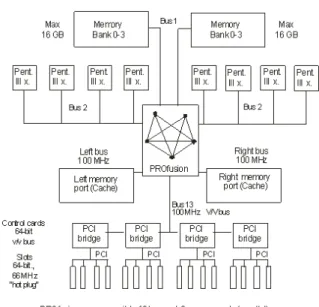
3.1. Symmetrical Multiprocessor System

Figure 2. Single computing node based on SMP (8-processors Intel Xeon).

Symmetrical multiprocessor system (SMP) is a multiple using of the same processors or cores which are implemented on motherboard in order to increase the whole

performance of such system. Typical common

characteristics are following

each processor or core (computing node) of the multiprocessor system can access main memory (shared memory)

I/O channels or I/O devices are allocated to individual computing nodes according their demands

integrated operation system coordinates cooperation of whole multiprocessor resources (hardware, software etc.).

Real example of multiprocessor system illustrates Fig. 2.

3.2. Network of Workstations

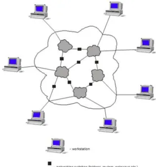
Network of workstations belongs to actually dominant trends in parallel computing. This trend is mainly driven by the cost effectiveness of such systems as compared to massive multiprocessor systems with tightly coupled processors and memories (supercomputers). Parallel computing on a network of workstations connected by high speed networks has given rise to a range of hardware and network related issues on any given platform [20, 35]. With the availability of cheap personal computers, workstations and networking devises, the recent trend is to connect a number of such workstations to solve computation intensive tasks in parallel on such clusters. Network of workstations has become a widely accepted form of high performance computing (HPC). Each workstation in a NOW is treated similarly to a processing element in a multiprocessor system. However, workstations are far more powerful and flexible than processing elements in conventional massive multiprocessors (supercomputers).

Typical example of networks of workstations also for solving large computation intensive problems is at Fig. 3. The individual workstations are mainly extreme powerful personal workstations based on multiprocessor or multicore platform [8, 18].

Figure 3. Typical architecture of NOW.

On such modular parallel computer we are able to study basic problems in parallel computing (parallel and distributed computing) as load balancing, inter processor communication IPC [22, 28], modeling and optimization of parallel algorithms etc. [10, 23, 26]. The coupled

computing nodes PC1, PC2, ..., PCi (workstations) could be

3.3. Massive Parallel Computers

3.3.1. Grid Systems

Grid technologies have attracted a great deal of attention recently, and numerous infrastructure and software projects have been undertaken to realize various versions of Grids. In general Grids represent a new way of managing and organizing of computer networks and mainly of their deeper resource sharing. Conceptually they go out, similar like computer networks, from a structure of virtual computer based on computer networks.

Figure 4. Architecture of Grid node.

Grid systems are expected to operate on a wider range of other resources as processors (CPU), like storages, data modules, network components, software (typical resources) and atypical resources like graphical and audio input/output devices, sensors and so one (Fig. 4.). All these resources typically exist within nodes that are geographically distributed, and span multiple administrative domains. The virtual machine is constituted of a set of resources taken from a resource pool. It is obvious that existed HPC parallel computers (supercomputers etc.) could be a member of such Grid systems too [31]. In general Grids represent a new way of managing and organizing of computer networks and mainly of their deeper resource sharing [34]. Grid systems are expected to operate on a wider range of other resources as processors (CPU), like storages, data modules, network components, software (typical resources) and atypical resources like graphical and audio input/output devices, sensors and so one (Fig. 4.). All these resources typically exist within nodes that are

geographically distributed, and span multiple

administrative domains. The virtual machine is constituted of a set of resources taken from a resource pool [34]. It is

obvious that existed HPC parallel computers

(supercomputers etc.) could be a member of such Grid systems too. In general Grids represent a new way of managing and organizing of computer networks and mainly of their deeper resource sharing.

3.3.2. Meta Computers

This term define massive parallel computer

(supercomputer, Grid) with following basic characteristics [8, 34]

wide area network of integrated free computing resources. It is a massive number of interconnected

networks, which are connected through high speed connected networks during which time whole massive system is controlled with network operation system, which makes an illusion of powerful computer system (virtual supercomputer) grants a function of meta computing that means

computing environment, which enables to

individual applications a functionality of all system resources

system combines distributed parallel computation with remote computing from user workstations. The best example of existed meta computer is Internet as massive international network of various computer networks according Fig. 5.

Figure 5. Internet as network of connected networks.

4. Analytical Performance Evaluation of

Parallel Computers

nasty problem, but there have been developed some solutions.

The second serious problem is blocking as consequence of always real limited technical resources. If one node is blocked, the node feeding could not enter more data into that node. Consider a communication network in which you are given the location of computing nodes and the required communication traffic between pairs of computing nodes. Then according mentioned theorem says that if you have Poisson traffic into an exponential server you get Poisson traffic out; but a message maintains its length as it passes through the network, so the service times are dependent as it goes along its path. Thus, one thing we want to do is to get rid of that dependence. We can do this by making an independence assumption; we just assume that the dependence does not exist. We manage this by allowing the communication message to change its length as it passes through the communication network. Every time it hits a new computing node, we are going to randomly choose the message length so that we come up with an exponential distribution again. With that assumption, we can then solve the queuing problem of communication in parallel computers. Let us assume infinite storage at all points in the network of coupled computing nodes and refer to the problem M/M/1, where the question mark refers to the modified input process. We then run simulations, with and without the independence assumption for a variety of networks. The reason why it is good to do it is that a high degree of mixing takes place in a typical communication network; there are many ways into a node and many ways out of the node [6, 16].

The assumption of independence permits us to break also the massive parallel computer into independent computing nodes, and allowed all node analysis to take place. The reason we had to make that assumption was because the communication message maintains the same length as they pass through the network. If we accept the independence assumption, it turns out that the queuing theory contains a number of results for cases where the service at a node is an independent random variable in an arbitrary network of queues. A basic theorem is due to Jackson [17, 29]. Jackson’s result essentially gives us the probability distribution for various numbers of messages at each of the nodes in such a network.

5. Application of Queuing Theory

The basic premise behind the use of queuing models for computer systems analysis is that the components of a computer system can be represented by a network of servers (resources) and awaiting lines (queues). A server is defined as an entity that can affect, or even stop, the flow of jobs through the system. In a computer system, a server may be the CPU, I/O channel, memory, or a communication port. Awaiting line is just that: a place where jobs queue for service. To make a queuing model work, jobs or customers or communication message (blocks

of data, packets) or anything else that requires the sort of processing provided by the server, are inserted into the network. A basic simple example could be the single server abstract model as single queuing theory system. In such model, jobs arrive at some rate, queue for service on a first-come first-served basis, receive service, and exit the system. This kind of model, with jobs entering and leaving the system, is called an open queuing system model [7, 27]. Queuing theory systems are classified according to various characteristics, which are often summarized using Kendall`s notation [3, 6]. The basic parameters of queuing theory systems are as following

λ - arrival rate at entrance to a queue

m- number of identical servers in the queuing system

ρ - traffic intensity (dimensionless coefficient of

utilization)

q - random variable for the number of customers in a system at steady state

w - random variable for the number of customers in a queue at steady state

E(ts)- the expected (mean) service time of a server

E(q)- the expected (mean) number of customers in a system at steady state

E(w) - the expected (mean) number of customers in a queue at steady state

E(tq) - the expected (mean) time spent in system

(queue + servicing) at steady state

E(tw) - the expected (mean) time spent in the queue

at steady state.

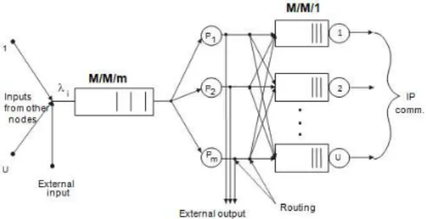
Communication demands (parallel processes, IPC data) arrive at random at a source node and follow a specific route in the communication networks towards their destination node. Data lengths of communicated IPC data units (for example in words) are considered to be random variables following distributions according Jackson theorem. Those data units are then sent independently through the communication network nodes towards the destination node. At each node a queue of incoming data units is served according to a first-come first-served (FCFS) discipline.

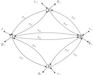
At Fig. 6 we illustrate generalization of any parallel computer including their communication network as following

computing nodes ui (i=1, 2, 3, ..., U) of any parallel

computer are modeled as graph nodes

network communication channels are modeled as

graph edges rij (i≠j) representing communication

intensities (relation probabilities).

The other used parameter of such abstract model are defined as following

u

γ

γ

γ

₁

,

₂

,

...

,

represent the total intensity of

input data stream to individual network computing nodes (the summary input stream from other connected computing nodes to the given i-th computing node. It is given as Poisson input stream

with intensity λi demands in time unit

ij

r

are given as the relation probabilities from node

i to the neighboring connected nodes j

u 2 1,β ,....,β

β correspond to the total extern output

stream of data units from used nodes (the total output stream to the connected computing nodes of the given node).

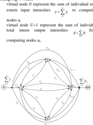
The created abstract model according Fig. 6 belongs in queuing theory to the class of open queuing theory systems (open queuing networks). Formally we can adjust abstract model adding virtual two nodes (node 0 and node U+1 according Fig. 7 where

virtual node 0 represent the sum of individual total

extern input intensities

_∑

=

= U

i i 1

γ

γ to computing

nodes ui

virtual node U+1 represent the sum of individual total intern output intensities

∑

=

= U i

i

1

β

β from

computing nodes ui.

Figure 7. Adjusted abstract model.

Such a model corresponds in queuing theory to the model of open servicing network. Adjective ”open” characterize the extern input and output data stream to the

servicing transport network [3, 29]. In common they are the open Markov servicing networks, in which the demand are mixed together at their output from one queuing theory system to another connected queuing theory system in a random way to that time as they are leaving the network. To the given i-th node the demand stream enter extern (from the network side), with the independent Poisson

arrival distribution and the total intensity

γ

i demands in

seconds. After servicing at i-th node the demand goes to the

next j-th node with the probability rij in such a way that the

demand walks to the j-th node intern (from the sight network). At this time the demand departures from i-th node to the other nodes are defined with probability

∑

= − U

j ij

r

1 1

6. Modeling of the NOW and Grid

NOW is a basic module of any Grid parallel computer. Structure of essential parts in any workstation (i-th node) of NOW based on single processor (m=1) or multiprocessor system (m - processors or cores) is illustrated at Fig. 8. Inter process communication (IPC) represents all needed communication in NOW as

communication among parallel processes control communication.

Figure 8. Structure of i – th computing node (WSi).

In principle we are assumed any constraints on structure of communication system architecture. Then we are modeling one workstation as a system with two dominant overheads

computation execution time [2] communication latency [23].

To model these overheads through applying queuing theory we created mathematical model of one i-th computing node according Fig. 9, which models

computation activities (processor’s latency) as one queuing theory system

every communication channel of i-th node LIi i = 1,

2, …, U as second queuing theory systems (communication latency).

6.1. Standard Analytical Model Based on M/M/M Queuing Systems

Let U be a node number of the whole transport system. For every node of NOW (i-th node according Fig. 10) we define the following parameters

λi - the whole number of incoming demands to the

i-th node, that is the sum both of external and

internal inputs to the i-th node

_∑

= = U i i 1 γ γ represent

the sum of individual total extern intensities in the NOW

λij - the whole input flow to the j-th communication

channel at i-th node

E(tq)i - the average servicing time in the program

queue (the waiting in a queue and servicing time) in the i-th node

E(tq)ij - the average servicing time of the j-th queue

of the communication channel (the queue waiting time and servicing time) at i-th node.

Figure 10. Standard analytical model of i-th computing node.

Then the whole extern input flow to the transport network is given as

∑

= = U i i 1 γ γ and i u i ij

i λ β

λ =

∑

+

=1

where βi represents the intern output from i-th node

(finished parallel programs in this node) which is not

further transmitted and is therefore not entering to the (LO)i.

Then the whole delay we can modeled as

                ⋅ + ⋅ =

∑

∑

= = U i u j ij q ij i q i now q i t E t E t E 1 1 ) ( ) ( 1 )

( λ λ

γ

, where

γ

λi⋅E(tq)i _and

γ λij⋅E(tq)ij

define individual contribution of computation queue delay (M/M/m) and communication channel delay (M/M/1) of

every node to the whole delay. For establishing E(tq)i for

computation queue delay it is necessary to know λi as the

whole intensity of the input flow to the message queue

where λ_i=γ_i+ all intern inputs flow to i-th node. The

intern input flow to i-th node is defined as the input from other connected nodes. We can express it in two ways

through solving a system of linear equations in

matrix form as λ =γ +λ⋅R

using of two data structures in form of tables and that is the routing table (RT) and destination probability tables (DPT).

In related model the routing table creates deterministic logical way from source i to the destination j. Concretely RT(i,j) has index (1, ..., N) of the next node on the route from i to j. This assumption of the fixed routing is not rare. We have proved also experimental, that the fix routing produces good analytical results in comparison to the alternate adaptive routing in a concrete communication network. The destination probability table destiny for each i, j pair the probability, that the message which outstands in node i is destined for node j. This table with n x n dimension and elements DPT(i, j) terminates which fraction

of the whole extern input

γ

i has the destination j, that is

) , (i j DTP

i⋅

γ . A path through the transport network we

can define as the sequence (x1, x2, ... , xm) in which

exist physical communication channel, which

connects x_k a x_k1,k =1,2, ...,m -1

k

j

k

j,

,

a

_k

∀

≠

j

x

x

(they do not exist loops).

We can define path with record ”path (j→k, i)” as

expression of the ordered sequence nodes, which are on the route from node j to the node k and they pass step by step

through nodes i. That is xi=j, xm=k, xp=i and

m p ≤

<

1 .

We define then

∑

→ ∈ U i k j path k ( ,)

as the summation over the

set of all destination nodes k so that node i lies on the route from the source node j. Then we get the relation for the

intern input flow to the i-th computing node

λ

i as follows

) , ( 1 1 k j DTP U j U k j⋅

∑ ∑

= =

γ , for j ≠ i,k∈path (j→ k,i)

and whole input flow to node i as

i). k, (j path k , ) , ( 1 1 → ∈ ≠ ⋅ + =

∑∑

= = i j for k j DTP U j U k i i

i γ γ

λ

We supposed also that the incoming demands are exponential distributed and that queue servicing algorithm

is FIFO (First In First Out). The program queue PQi is

servicing through one or more the same computation processors, which performed incoming demands (parallel processes). In demand servicing in a given node could be two possibilities

demand is in the addressed node and she will leave communication network.

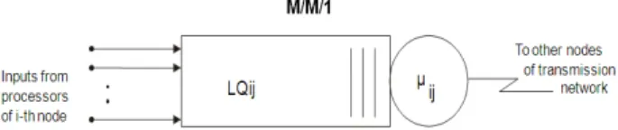
To every communication channel is set the queue of the given communication lines (LQ), which stores the demands (their pointers) who are awaiting the communication through this communication channel. Also in this case we supposed its unlimited capacity, exponential inter arrival time distribution of input messages and the servicing algorithm FIFO. Every communication line queue has its

communication capacity Sij (in data units per second).

Because we supposed the exponential demand length distribution the servicing time is exponential distributed too

with average servicing time 1/ µ Sij, where µ is the average

message length and Sij is the communication capacity of

node i and of communication channel j. For simplicity we

will assume, as it is obvious, that Sij is a part of µ. To find

the average waiting time in the queue of the communication system we consider the model of one communication queue part node as M/M/1 queuing theory system according Fig. 11.

Figure 11. Model of one M/M/1 communication channel of the i-th node.

The total incoming flow to the communication channel j

at node i which is given through the value

λ

ij and we can

determine it with using of routing table and destination

probability table in the same way as for the value

λ

i. Then

ρij as the utilization of the communication channel j at the

node i is given as

ij ij ij S

µ

λ

ρ

=

The total average delay time in the queue E(tq)i is

ij ij ij q t E

λ

µ

− = 1 ) (

If we now substitute the values for Ti and Tij to the

relation for T we can get finally the relation for the total average delay time of whole transport system as

                − ⋅ + − ⋅ =

∑

∑

= = U i u

j ij _ij

ij i i i now q i t E 1 1 1 1 1 ) ( λ µ λ λ µ λ γ

6.2. Model with M/D/m and M/D/1 Systems

The used model were built on assumptions of modeling incoming demands to program queue as Poisson input stream and of the exponential inter arrival time between communication inputs to the communication channels. The idea of the previous models were the presumption of decomposition to the individual independent channels

together with the independence presumption of the demand length, that is demand lengths are derived on the basis of

the probability density function pi = µ e-µt for t > 0 and f(t)

= 0 for t ≤ 0 always at its input to the node. On this basis it

was possible to model every used communication channel as the queuing theory system M/M/1 and to derive the average value of delay individually for every channel too. The whole end-to-end delay was then simply the sum of the individual delays of the every used communication channel.

These conditions are not fulfilled for every input load, for all architectures of node and for the real character of processor service time distributions. These changes could cause imprecise results. To improve the mentioned problems we suggested the behavior analysis of the modeled NOW module improved analytical model (Fig. 12), which will be extend the used analytical model to more precise analytical model supposing that

we consider to model computation activities in every node of NOW network as M/D/m system we consider an individual communication channels in i-th node as M/D/1 systems. In this way we can take into account also the influence of real non exponential nature of the inter arrival time of inputs to the communication channels.

These corrections may to contribute to precise behavior

analysis of the NOW network for the typical

communication activities and for the variable input loads. According defined assumption to modeling of the computation processors we use the M/D/m queuing theory systems according Fig. 12. To find the average program queue delay we have used the approximation formula for M/D/m queuing theory system as follows

        ⋅ ⋅ − ⋅ − ⋅ − + = ) / / ( ) ( ) 1 / / ( ) ( ) 1 / / ( ) ( 16 2 45 ) 1 ( ) 1 ( 1 ) / / ( ) ( i w w w i i i i i i w m M M t E M M t E D M t E m m m m D M t E ρ ρ

, in which

ρi - is the processor utilization at i-th node for all

used processors

mi - is the number of used processors at i-th node

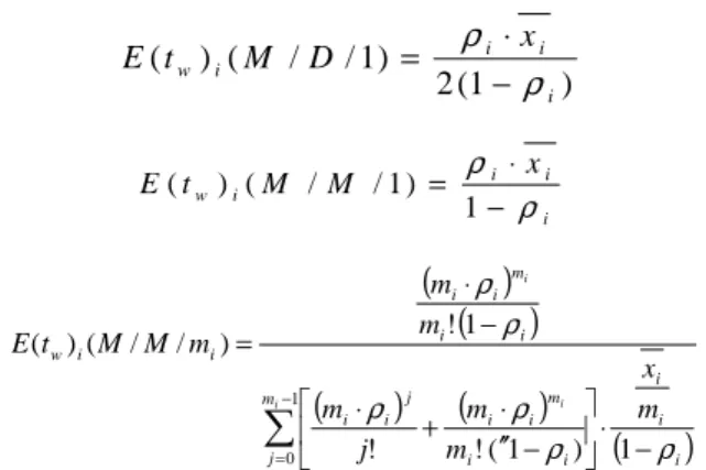
E(tw)(M/D/1), E(tw) (M/M/1) and E(tw) (M/M/m)

are the average queue delay values for the queuing theory systems M/D/1, M/M/1 and M/M/m respectively.

The chosen approximation formulae we selected from two following points

for his simply calculation

if the number of used processors equals one the used relation gives the exact solution, that is W(M/D/1) system. Such number of processors is often used in praxis

if the number of processors greater than one (mi > 1)

the used relation generate a relative error, which is not greater as 1%. This fact we verified and confirmed through simulation experiments.

Let x define the fixed processing time of the i-th node _i

processors and E(tw)i (PQ) the average program queue

delay in the i-th node. Then ρi, as the utilization of the i-th

node, is given as

i i i i m x . λ ρ =

Then the average waiting time in PQ queue

E(tw)i(M/D/mi) is given trough the following relations

) 1 ( 2 ) 1 / / ( ) ( i i i i w x D M t E

ρ

ρ

− ⋅ = i i i i w x M M t E ρ ρ − ⋅ = 1 ) 1 / / ( ) (

By substituting relations for ρi, E(tw)i (M/D/1), E(tw)i

(M/M/1) and E(tw)i (M/M/mi) in the relation for E(tw)I

(M/D/mi) we can determine E(tw)I (PQ). Then the total

average delay for the communication activities in i-th node is simply the sum of average message queue delay (MQ) plus the fixed processing time

i i

w i

w E t PQ x

t

E( ) = ( ) ( )+

To find the average waiting time in the queue of the communication system we consider the model of one communication queue part node as M/M/1 queuing theory system according

Fig. 11. Let x_ij determine the average servicing time

for channel j at the node i. Then ρij as the utilization of the

communication channel j at the node i is given as

ij ij ij ij

S

x

λ

ρ

=

where Sij is the communication channel speed of j-th

node. For simplicity we will assume that Sij = 1. The total

incoming flow to the communication channel j at node i

which is given through the value

λ

ij and we can determine

it with using of routing table and destination probability

table in the same way as for a value

λ

i. Let E(tw)ij (LQ) be

the average waiting queue time for communication channel j at the node i. Then

) 1 ( ) ( ) ( ij ij ij ij w x LQ t E ρ ρ − ⋅ =

The total average delay value is the queue E(tw)ij is given

then as

There If we now substitute the values for E(tq)i and E(tq)ij

to the relation for E(tq)now we can get finally the relation for

the total average delay time of whole NOW model is given as

(

) (

)

_       + + + =

∑

∑

= = U i u j ij ij w i i w now q i x LQ t E x PQ t E t E 1 1 ) ( ) ( ) ( ) ( 1 ) ( γ

6.3. Mixed Analytical Models

6.3.1. Analytical Model with M/M/m and M/D/1 Queuing Systems

This model is mixture of analyzed model. The first part

of final total average time E(tq)i we get from chapter 6.1

and second part from 6.2.1 one. Then for E(tq)now we can

get finally

6.3.2. Model with M/D/m and M/M/1 Queuing Systems In this model the first part of final total average time

E(tq)i we can also get from chapter 6.2.1 and second part

from 6.1 respectively. Then for E(tq)now we get for this

model finally

(

)

_               − ⋅ + + =

∑

∑

= = U i u

j ij _ij

ij i i w now q i x PQ t E t E 1 1 1 ) ( ) ( 1 ) ( λ µ λ γ

6.3.3. Analytical Model of Massive Grid Parallel Computers

We have defined Grid system as network of NOW network modules. Let N is the number of individual NOW networks or similar clusters. Then final total average time E(tq)grid

      =

∑

= N i now i q grid

q E t

t E 1 ) ( 1 ) ( α where

∑

= = N i i 1 γ

α represent the sum of individual total extern

intensities to the i-th NOW module in the Grid

(

)

(

)

(

)

(

)

(

i

)

i i m

j i i

m i i j i i i i m i i i i w m x m m j m m m m M M t E i i i ρ ρ ρ ρ ρ ρ − ⋅       − ′′ ⋅ + ⋅ − ⋅ =

∑

−

= ! !(1 ) 1

E(tq)i now correspondent to individual average times

in i- th NOW module (i=1, 2, … N).

The intern input flow to i-th node is defined as the input from all other connected computing nodes. We can express it in two following ways

through solving a system of linear equations in

matrix form as

λ

=

γ

+

λ

⋅R

using of two data structures in form of tables and that is the routing table (RT) and destination probability tables (DPT).

To improve the mentioned problems we suggested improved analytical model, which extends the used standard analytical model to more precise analytical model (improved analytical model) supposing that

we consider to model computation activities in every node of NOW network as M/D/m system (assumption input of balanced parallel processes to every node)

we consider an individual communication channels in i- th node as M/D/1 systems. In this way we can take into account also the influence of real non exponential nature of the inter arrival time of inputs to the communication channels.

Both analyzed analytical models are not fulfilled for every input load, for all parallel computer architectures and for the real character of computing node service time distributions. These changes may cause at some real cases imprecise results. Another survived problem of the used standard analytical model is assumption of the exponential inter arrival time between message inputs to the

communication channels in case of unbalanced

communication complexity of parallel processes. To remove mentioned changes we derived a correction factor to standard analytical model.

7. Corrected Standard Analytical Model

The derived standard analytical model supposes that the inter arrival time to the node’s communication channels has the exponential distribution. This assumption is not true mainly in the important cases of high communication utilization. The node servicing time of parallel processes (computation complexity) could vary from nearly deterministic (in case of balanced parallel processes) to exponential (in case of unbalanced ones). From this in case of node’s high processors utilization the outputs from individual processor of node’s multiprocessor may vary from the deterministic interval time distribution to exponential one. These facts violate the assumption of the random exponential distribution and could lead to erroneous value of whole node’s delay calculation. Worst of all this error could the greater the higher is the node utilization. From these causes we have derived the correction factor which accounts the measure of violation for the exponential distribution assumption.

The inter arrival input time distribution to each node’s

communication channel depends on ρi, where ρi is the

overall processor utilization at the node i. But because only

the part

λ

ij from the total input rate

λ

i for node i go to the

node’s communication channel j, it is necessary to weight the influence measure of the whole node’s processors

utilization trough the value

λ

ij /

λ

ij for channel j as

)

/

(

_{ij i}

i

λ

λ

ρ

⋅

To clarify the node’s processor utilization influence to the average delay of communication channel we have tested the 7-noded experimental parallel computer. The processing time was varied to develop the various workloads of node’s processors.

Extensive testing have proved, that if we increase utilization of communication channel and that develops saturation of communication channel queue then average queue waiting time is less sensitive to the nature of inter arrival time distributions. This is due to the fact that the messages (communicating IPC data) wait longer in the queue what significantly influenced the increase of the average waiting time and the error influence of the non-exponential inter arrival time distribution is decreased. To incorporate this knowledge for the correlation factor we

investigated the influence of the weighting pi(λij/λi)

through the value x

ij)

1

( −ρ for various values x. The

performed experiments showed the best results for the value x = 1. Derived approximation of the average queue waiting time of the communication channel j at the node i, which eliminates violence of the exponential inter arrival time distribution is then given as

i ij ij i

λ λ ρ ρ ⋅(1− )⋅

The finally correction factor of the communication

channel j at the node i, which we have named as cij is as

following

i ij ij i ij

c

λ λ ρ

ρ ⋅ − ⋅

−

=1 (1 )

With the derived correction factor cij we can define now

the corrected average queue waiting time as:

) ( )

(

' LQ c W LQ

Wij = ij⋅ ij

The standard analytical model we can simply correct in

such a way that instead of Wij(LQ) we will consider its

corrected value Wij’(LQ). In this way derived improved

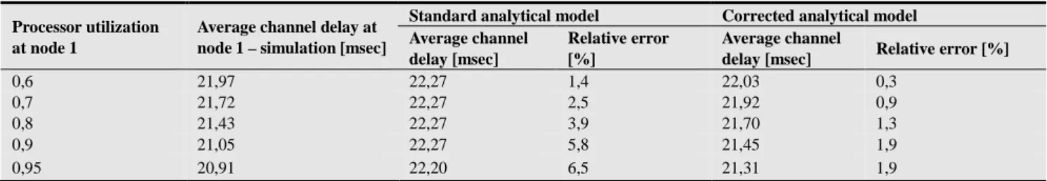
Table 1. Achieved results for correction factor

Processor utilization at node 1

Average channel delay at node 1 – simulation [msec]

Standard analytical model Corrected analytical model

Average channel delay [msec]

Relative error [%]

Average channel

delay [msec] Relative error [%]

0,6 21,97 22,27 1,4 22,03 0,3

0,7 21,72 22,27 2,5 21,92 0,9

0,8 21,43 22,27 3,9 21,70 1,3

0,9 21,05 22,27 5,8 21,45 1,9

0,95 20,91 22,20 6,5 21,31 1,9

20 20,5 21 21,5 22 22,5

0,6 0,7 0,8 0,9 0,95

Node channel delay for simulation [msec] Node channel delay for standard model [msec] Node channel delay for corrected model [msec]

Figure 13. The influence of the exponential time distribution and its

correction.

The average delay values of the node’s communication channel achieved through simulation are compared with the results of the standard analytical model (exponential inter arrival time distribution) and with the results of the corrected standard model. Comparison of the relative errors is illustrated in the Fig. 14.

0,6

0,7 _0,8

0,9 _0,95 0

1 2 3 4 5 6 7

Relative error of corrected model [%]

Relative error of standard model [%]

Figure 14. Comparison of relative errors.

At Table 2 there are results of the channel utilization

influence to the average waiting time for the

communication channel of 7 - noded communication network. For this case the channel utilization was influenced through communication speed changes.

Table 2. The results of the channel influence

Processor

utilization at node 1

Average channel delay for node 1 using simulation [msec]

Standard analytical model Corrected analytical model

Average channel delay [msec]

Relative error [%]

Average channel delay [msec]

Relative error [%]

0,6 8,89 9,25 4,1 8,68 2,4

0,7 15,92 16,38 2,9 15,91 0,06

0,8 31,04 31,94 2,9 31,39 1,1

0,9 79,76 81,08 1,7 80,38 0,8

The achieved results in Table 2 are illustrated at Fig. 15 including their relative errors related to simulation results.

The influence of communication channel utilization to the result accuracy of the analytical models is at the Fig. 16. From these achieved results follow that decreasing of the node’s communication channel utilization the difference between simulated results and the standard analytical model increases.

Figure 16. Influence of channel utilization to the accuracy of analytical

models.

8. Other Achieved Results

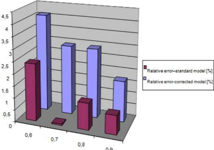
Table 3 represents results and relative errors for the average value of the total message delay in the 5 nodes communication network so for classical analytical model (M/M/m + M/M/1) as for developed more precise analytical model (M/D/m + M/D/1) in which for multiprocessor’s node activities we consider very real fixed latency. The same fixed delay was included to the average communication delay at each node and in simulation model

too. These assumptions correspondence to the same communication speeds in each node’s communication channel. If used communication channels do not have the same communication speeds then communication latencies are different constants. In both considered analytical models (M/M/m + M/M/1, M/D/m + M/D/1) performed experiments have proved that decreasing of processor

utilization ρ cause decreasing of total average delay in

NOW module E(tq)now. Therefore parallel processes are

waiting in parallel processes queues shorter time. In contrary decreasing of node’s communication channel speed increase communication channel utilization and then data of parallel processes have to wait longer in communication channel queues and increase the total node’s latency. Tested results have also proved the influence of real non exponential nature of the input inter-arrival time to node’s communication channels. In relation to it the analytical model M/D/m + M/D/1 provides best results and the analytical model M/M/m + M/M/1 the worst ones. The results for other possible mixed analytical models (M/M/m + M/D/1, M/D/m + M/M/1) provide results between the best and worst solutions. For simplicity deterministic time to perform parallel processes at node’s multiprocessor activities (the servicing time of PQ queue)

was settled to 8µs and the extern input flow for each node

was the same constant too.

Table 3. Comparison of considered analytical models

Processor utilization

Whole delay for simulation [msec]

Standard analytical model Corrected analytical model

End -to- end delay [msec] Relative error [%] End –to- end delay [msec] Relative error [%]

0,2 21,45 20,06 6,48 20,83 2,89

0,3 23,53 21,58 8,29 22,85 2,89

0,4 26,24 23,49 10,48 25,51 2,78

0,5 30,16 26,51 12,10 29,44 2,39

0,6 34,69 29,79 14,12 33,92 2,22

0,7 41,67 35,19 15,55 41,38 0,70

0,8 54,25 44,08 18,75 54,43 0,33

0,9 80,01 60,38 24,53 84,47 6,82

To vary the processor utilization we modified the extern input flow in the same manner for each used node. Comparison of whole delay illustrates for both tested analytical models (standard, corrected) in relation to simulated results are presented at Fig. 17.

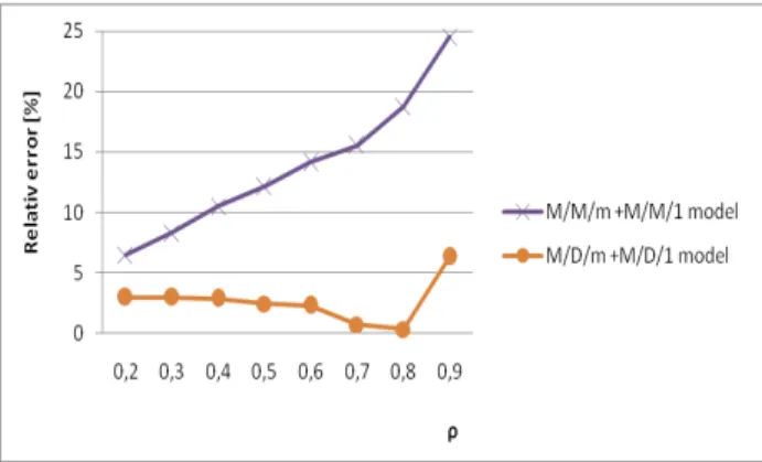
To vary node’s processor utilization we modified the extern input flow in the same manner for each node of NOW module. For both analytical models (the best and the worst cases) are at Fig. 18 the relative errors in relation to simulation results. The best analytical model (M/D/m + M/D/1) provides very precision results in the whole range of input workload of multiprocessors and every communication channel’s utilization with relative error, which does not exceed 6.2% and in most cases are in the range up to 5%. This is very important to project heavily loaded NOW network module (from about 80 to 90%), where the accurate results are to be in bad need of to avoid any bottleneck congestions or some other system instabilities.

Figure 18. Relative errors of analyzed models.

The relative errors of worst analytical model are from 7 to 25%. This is due influences of processes queues delays, the nature of inter arrival input to the communication channel in the case of high processor utilization. In contrary the corrected analytical model in all cases has the relative number not greater than 7%. The achieved results in Table 3 indicate also other important critical fact. The derived corrected model produces more precise results in the whole range of node’s processor utilization including the range of their higher utilization (in range 0,5 – 0,9) which are the most interesting to practical use. All developed analytical models could be applied also for large NOW networks practically without any increasing of the computation time in comparison to simulation method because of their explained module’s structure based on NOW module. Simulation models require oft three orders of magnitude more computation time for testing massive meta computer. Therefore limiting factor of the developed analytical models will not be computation complexity, but space complexity of memories for needed RT and DPT tables.

These needed RT and DPT tables require O(n2) memory

cells, thus limiting the network analysis to the number of N nodes about 100 - 200 for the common SMP multiprocessor. In case of possible solving system of linear equations to

find in analytical way node’s λi and λij, most parallel

algorithms use to its solution Gauss elimination method (GEM). Used GEM parallel algorithms have computation

complexity as O(n3) floating point multiplications and a

similar number of additions [2, 15]. These values are however adequate to handle most existing communication network. In addition to it also for any future massive meta computers we would be always used hierarchically modular architecture, which consist on such simpler NOW modules.

We also point out, that accuracy contribution of corrected analytical model was achieved without the increasing the computation time in comparison to standard analytical model. It is also remarkable to emphasize increasing influence of the simulation complexity for the analysis of

real massive parallel computers including their

communication networks. The simulation models require three orders of magnitude more computation time for testing such complex parallel systems.

9. Conclusion

Performance evaluation of computers generally used to be a very hard problem from birthday of computers. This involves the investigation of the control and data flows within and between components of computers including their communication networks. The aim is to understand the behavior of the systems, which are sensitive from a performance point of view [32, 33]. It was, and still remains, not easy to apply any analytical method (queuing theory, theory of complexity, Petri nets) to performance evaluation of parallel computers because of their high number of not predictable parameters [21, 25]. Using of actual parallel computers (SMP -multiprocessor, multicore, NOV, Grid) open more possibilities to apply a queuing theory results to analyze more precise their performance. This imply existence of many inputs streams (control, data), which are inputs to modeled queuing theory systems and which are generated at various used resources by chance

(assumption for good approximation of Poisson

distribution). Therefore we could model computing nodes of parallel computers as M/D/m or M/M/m and their communication channels as M/D/1 or M/M/1 queuing theory systems in any existed parallel computer (SMP, NOW, Grid, meta computer).

Applied using of such flexible analytical modeling tool based on queuing theory results) shows real paths to a very effective and practical performance analysis tool including massive parallel computers (Grid, meta computers). In summary developed more precise analytical models could be applied to performance modeling of dominant parallel computers and that in following typical cases

single computing nodes based on SMP parallel computer (multiprocessors, multicores, mix of them)

NOW based on workstations (single, SMP) Grid (network of NOW modules)

mixed parallel computers (SMP, NOW, Grid) meta computer (massive Grid).

From a point of user application of any analytical method is to be preferred in comparison with other possible methods, because of its universal and transparent character. Therefore the developed analytical models we can apply to performance modeling of any parallel computer or some parallel algorithms too (overheads). To practical applied using of developed analytical model we would like to advise following

running of unbalanced parallel processes where λ is

a parameter for incoming parallel processes with

their exponential service time distribution as E(ts) =

1/µ (corrected standard model)

recalculate them to such units at first node entrance we would like to refer in next paper

running of parallel processes (λ parameter for

incoming parallel processes with their deterministic

service time E(ts) = 1/µ = constant). The

deterministic servicing times are a very good approximation of balanced parallel processes

(M/D/m) with nearly equal amount of

communication data blocks for every parallel process (M/D/1)

in case of using analytical model using M/D/m

and M/D/1 we can consider λ parameter also for

incoming units of parallel processes (data block, packet etc.) with their average service time for

considered unit ti, where E(ts) = 1/µ = ti =

constant.

Using developed analytical models we are able to apply them so to both traditionally parallel computers (massive SMP) as distributed computers (NOW, Grid, meta computer). In such unified parallel computer models we are able better to study load balancing, mixed inter process communication IPC (shared and distributed memory),

communication transport protocols, performance

optimization and prediction in parallel algorithms etc. We would also like to analyze nasty problems in parallel computing as follows

blocking problem (exhausted limited shared resources)

waiting time T(s, p)wait as blocking consequence [11,

12]

influence of routing algorithms

to prove, or to indicate experimentally, the role of the independence assumption, if you are looking for higher moments of delay

to verify the suggested model also for node limited buffer capacity and for other servicing algorithms than assumed FIFO (First In First Out)

unified grouped decomposition models for parallel and distributed computing [13, 15]

intensive testing, measurement and analysis to estimate technical parameters of used parallel computers [5, 24].

Acknowledgements

This work was done within the project “Complex modeling, optimization and prediction of parallel computers and algorithms” at University of Zilina, Slovakia. The author gratefully acknowledges help of project supervisor Prof. Ing. Ivan Hanuliak, PhD.

References

[1] Abderazek A. B., Multicore systems on chip - Practical Software/Hardware design, Imperial college press, United Kingdom, pp. 200, 2010

[2] Arora S., Barak B., Computational complexity - A modern Approach, Cambridge University Press, UK, pp. 573, 2009

[3] Dattatreya G. R., Performance analysis of queuing and computer network, University of Texas, Dallas, USA, pp. 472, 2008

[4] Dubois M., Annavaram M., Stenstrom P., Parallel Computer Organization and Design, Cambridge university press, United Kingdom, pp. 560, 2012

[5] Dubhash D.P., Panconesi A., Concentration of measure for the analysis of randomized algorithms, Cambridge University Press, UK, 2009

[6] Gelenbe E., Analysis and synthesis of computer systems, Imperial College Press, UK; pp. 324, 2010

[7] Giambene G., Queuing theory and telecommunications, Springer, pp. 585, 2005

[8] Hager G., Wellein G., Introduction to High Performance Computing for Scientists and Engineers, CRC Press, USA, pp. 356, 2010

[9] Hanuliak Peter, Hanuliak Michal, Modeling of single computing nodes of parallel computers, American J. of Networks and Communication, Science PG, Vol.3, USA, 2014

[10] Hanuliak J., Hanuliak I., To performance evaluation of distributed parallel algorithms, Kybernetes, Volume 34, No. 9/10, UK, pp. 1633-1650, 2005

[11] Hanuliak P., Analytical method of performance prediction in parallel algorithms, The Open Cybernetics and Systemics Journal, Vol. 6, Bentham, UK, pp. 38-47,2012

[12] Hanuliak P., Hanuliak I., Performance evaluation of iterative parallel algorithms, Kybernetes, Volume 39, No.1/ 2010, United Kingdom, pp. 107- 126, 2010

[13] Hanuliak J., Modeling of communication complexity in parallel computing, American J. of Networks and Communication, Science PG, Vol. 3, USA, 2014

[14] Hanuliak P., Complex analytical performance modeling of parallel algorithms, American J. of Networks and Communication, Science PG, Vol. 3, USA, 2014

[15] Hanuliak P., Hanuliak J., Complex performance modeling of parallel algorithms, American J. of Networks and Communication, Science PG, Vol. 3, USA, 2014

[16] Harchol-BalterMor, Performance modeling and design of computer systems, Cambridge University Press, United Kingdom, pp. 576, 2013

[17] Hillston J., A Compositional Approach to Performance Modeling, University of Edinburg, Cambridge University Press, United Kingdom, pp. 172, 2005

[18] Hwang K. and coll., Distributed and Parallel Computing, Morgan Kaufmann, USA, pp. 472, 2011

[19] Kshemkalyani A. D., Singhal M., Distributed Computing, University of Illinois, Cambridge University Press, United Kingdom , pp. 756, 2011

[21] Kostin A., Ilushechkina L., Modeling and simulation of distributed systems, Imperial College Press, United Kingdom, pp. 440, 2010

[22] Kumar A., Manjunath D., Kuri J., Communication Networking , Morgan Kaufmann, USA, pp. 750, 2004

[23] Kushilevitz E., Nissan N., Communication Complexity, Cambridge University Press, United Kingdom, pp. 208, 2006

[24] Kwiatkowska M., Norman G., and Parker D., PRISM 4.0: Verification of Probabilistic Real-time Systems, In Proc. of 23rd CAV’11, Vol. 6806, Springer, Germany, pp. 585-591, 2011

[25] Le Boudec Jean-Yves, Performance evaluation of computer and communication systems, CRC Press, USA, pp. 300, 2011

[26] McCabe J., D., Network analysis, architecture, and design (3rd edition), Elsevier/ Morgan Kaufmann, USA, pp. 496, 2010

[27] Meerschaert M., Mathematical modeling (4-th edition), Elsevier, Netherland, pp. 384, 2013

[28] Misra Ch. S.,Woungang I., Selected topics in communication network and distributed systems, Imperial college press, UK, pp. 808, 2010

[29] Natarajan Gautam, Analysis of Queues: Methods and Applications, CRC Press , USA, pp. 802, 2012

[30] Peterson L. L., Davie B. C., Computer networks – a systemapproach, Morgan Kaufmann, USA, pp. 920, 2011

[31] Resch M. M., Supercomputers in Grids, Int. J. of Grid and HPC, No.1, pp. 1 - 9, 2009

[32] Riano l., McGinity T.M., Quantifying the role of complexity in a system´s performance, Evolving Systems, Springer Verlag, Germany, pp. 189 – 198, 2011

[33] Ross S. M., Introduction to Probability Models, 10th edition, Academic Press, Elsevier Science, Netherland, pp. 800, 2010

[34] Wang L., Jie Wei., Chen J., Grid Computing: Infrastructure, Service, and Application, CRC Press, USA, 2009

www pages