THE IMPACT OF FUTURE CO2 EMISSION REDUCTION TARGETS
ON U.S. ELECTRIC SECTOR WATER USE
Colin MacKay Cameron
A thesis submitted to the faculty of the University of North Carolina at Chapel Hill in partial fulfillment of the requirements for the degree of Master of Science in the Department of
Environmental Sciences and Engineering.
Chapel Hill 2013
Approved by:
Dr. J. Jason West
Dr. Gregory Characklis
ii © 2013
iii
Abstract
COLIN MACKAY CAMERON: The Impact of Future CO2 Emission Reduction Targets on U.S. Electric Sector Water Use
(Under the direction of Dr. J. Jason West)
The U.S. electric sector’s reliance on water makes it vulnerable to the impacts of
climate change on water resources. Here we analyze how constraints on U.S. energy
system carbon dioxide (CO2) emissions could affect water withdrawal and consumption in
the U.S. electric sector through 2055. We use simulations of the EPA’s U.S. 9-region
(EPAUS9r) MARKAL least-cost optimization energy systems model with updated water use
factors for electricity generating technologies. Model results suggest CO2 constraints could
force the retirement of old power plants and drive increased use of low water-use
renewable and nuclear power as well as natural gas CCS plants with more advanced cooling
systems. These changes in electric sector technology mix reduce water withdrawal in all
scenarios but increase water consumption in aggressive scenarios. Decreased electric
sector water withdrawal would likely reduce electric sector vulnerability to climate change,
iv
Acknowledgements
I would like to thank my advisor Dr. J. Jason West for his advice, support and hours
of assistance with this research. I would also like to thank William Yelverton, Rebecca
Dodder, Carol Lenox, and Dan Loughlin for their patience, insight and generosity in teaching
v
Table of Contents
List of Figures…….……….vii
List of Abbreviations……..……….……….viii
Chapter I. Introduction………..1
II. Background………4
III. Methods………..7
MARKAL Model……….…………..7
Model Scenarios……….9
Water Use in Electricity Generation………..11
IV. Results………15
Model Response to Constraints by Sector………15
Electric Sector Technology Changes………..19
Electric Sector Technology Changes by Region……….23
Electric Sector Water Use……….28
V. Sensitivity Analysis……….33
Scenarios………..33
Results……….34
vi
VI. Conclusion………39
Appendix A: Regional Water Use Map……….……….………43
Appendix B: Net Flows of Embodied Water……….……….44
Appendix C: Water Use vs. Electricity Use by Region……….……45
vii
List of Figures
Figure
1. Water Withdrawal and Consumption Factors………….……….…14
2. System and Sector CO2 Emissions.………...……….………….…17
3. CO2 Emissions by Sector and Light Duty Vehicle Technologies………..….18
4. Electric Sector Technology Mix………21
5. Electric Sector Technology Mix by Region.………..…..26
6. Net Flows of Electricity..……….…..…..27
. 7. Electric Sector Water Use……….………..….……..31
8. Electric sector water withdrawal and consumption by region ………..………..32
9. Sensitivity Analysis. ………..………..38
10.Regional Water Use...………..………….43
11.Net Flows of Embodied Water……….………..………….44
viii
List of Abbreviations
AEO 2012 U.S. Department of Energy Annual Energy Outlook 2012 CAIR Clean Air Interstate Rule
CAFE Corporate Average Fuel Economy
CCS Carbon Capture and Sequestration
CO2 Carbon Dioxide
EIA Energy Information Administration
EPAUS9r Environmental Protection Agency United States Nine Region Database
H.R. U.S. House of Representatives
kWh Kilowatt Hour
MARKAL MARKet ALlocation energy systems model
MW Megawatt
MWh Megawatt Hour
NOx Nitrogen Oxides
NREL National Renewable Energy Laboratory
PJ Petajoule
ReEDS Regional Energy Deployment System RPS Renewable Portfolio Standard
SOx Sulfur Oxides
I.
Introduction
Over 90% of U.S. electricity supply is generated by thermoelectric power plants25
that require an abundant supply of water for cooling. The electric sector withdraws more
water than any other sector in the U.S.,29 accounting for 41% of all freshwater withdrawals.8
Electric sector water use also accounts for 6% of all water consumption in the U.S. and is
expected to grow to 9% by 2030, making it the fastest growing water consumer.1 This
heavy dependence on water means the U.S. electric sector is highly vulnerable to changes in
water resource availability; when cooling water supply is compromised, electricity
generation may be reduced or shutdown.9
Thermoelectric cooling can be compromised in three ways. First, the water level of
rivers and other cooling water sources can fall below the cooling water intakes of nearby
power plants and thereby prevent those plants from withdrawing sufficient water for
cooling. Second, high source water temperatures can reduce the efficiency of power plant
cooling systems and consequently limit electricity generating capacity.21 Finally, state
regulations prohibit power plants from discharging heated cooling water into water bodies
that already exceed temperature thresholds designed to protect water quality and
ecosystems.1 As a result, when water temperatures approach or exceed these limits, power
2
Over the last decade, droughts and heat waves have compromised cooling water
sources and disrupted power generation numerous times. One of the best-known incidents
was a widespread drought and heat wave that affected the southeastern United States in
August 2007. It forced multiple Tennessee Valley Authority (TVA) power plants, including
the 3,297 MW Brown’s Ferry nuclear plant, to temporarily curtail operations.9 TVA was
forced to buy power from neighboring utilities to meet electricity demand resulting in
considerable cost increases to consumers.31 Water limitations have forced similar power
generation reductions at multiple sites throughout the United States9 including as recently
as August of 2012 at the Millstone Nuclear Power Station in Waterford Connecticut.6
These episodes are likely to become more frequent and more severe in the future as
a result of climate change. Numerous climate modeling assessments have projected
significant decreases in average low stream flows17 and increases in average water
temperatures30 in many parts of the U.S. over the next 50 years. These changes are
projected to be most severe in the southern and southeastern U.S. where river
temperatures may exceed regulatory limits as often as 40 days per year and low stream
flows could decrease by an additional 25% by 2040.30 These changes have the potential to
reduce total U.S. electric generating capacity by as much as 16% over the next 20 to 40
years.30
This vulnerability to climate change may be further exacerbated by increased
demand for electricity and increased competition for water from other sectors in the future.
The Energy Information Administration (EIA) projects the U.S. will consume over 27% more
3
demand is met in the future, electric sector water use could increase or decrease because
of significant differences in the water use of electricity generating technologies and cooling
systems.12 Changes in electric sector water use influence its vulnerability to climate change,
as well as the availability of water for use in other sectors across the economy. In light of
the threat to U.S. electric power reliability, it will be critical to understand how future
energy policies could impact electric sector water use.
This study explores how energy policies aimed at mitigating climate change through
greenhouse gas emissions reductions could impact electric sector water use at a regional
level. Specifically, we evaluate how four scenarios of U.S. energy sector carbon dioxide
(CO2) emission reductions could impact the water use of the electric power sector through
2055 using simulations of the EPA’s U.S. 9-region (EPAUS9r) MARKAL (MARKet ALlocation)
energy systems model.19,11 Previous analysis has explored the effects on water use of CO2
emissions reduction in the electric sector alone using the ReEDS model.13 The advantage of
the MARKAL model is its ability to capture economic interactions between multiple sectors
of the energy system. In this analysis, MARKAL provides a cross-sector framework to
II.
Background
Thermoelectric power plants generate electricity by using steam to drive turbines.
These plants require cooling systems to condense turbine exhaust steam back into boiler
feed water. To meet this need, power plants divert water from nearby water bodies such as
rivers and lakes. Cooling water is then pumped through a heat exchanger to condense the
exhaust steam. Once cooling water has passed the heat exchanger, it is either discharged
back into the environment, or pumped through a cooling system (such as towers and
ponds) and recycled back into the condenser.
Water use is defined in terms of two parameters: withdrawal and consumption.
Water withdrawal at a thermoelectric power plant is the total amount of water diverted
from the environment. Water consumption is the amount of water lost as a result of the
cooling process primarily as a result of evaporation. Over 99% of cooling water is
withdrawn from surface water bodies, but some power plants also withdraw cooling water
from groundwater sources.29 In addition to freshwater, saline and brackish water is used to
meet some thermoelectric cooling needs in coastal areas.
The most significant determinant of a thermoelectric power plant’s water use is its
cooling system. Thermoelectric cooling systems are divided into five classes: once-through,
recirculating, pond, dry and hybrid. Once-through (or open-loop) cooling systems
5
the environment. Recirculating (or closed-loop) cooling systems use natural draft, forced
draft or induced draft cooling towers to dissipate waste heat through evaporation and
return the remaining water for further cooling use. As a result of this evaporative cooling
process, recirculating cooling systems consume on average twice as much water as
once-through cooling systems. However, recirculating cooling systems withdraw water only to
replace the losses from the cooling water reservoir and therefore withdraw 10 to 100 times
less water than a once-through cooling system.12
Pond cooling systems discharge heated cooling water into dedicated, open-air
cooling water reservoirs and return cooler water from the same pond back into the cooling
system. Dry cooling systems force air through the heat exchanger in place of water, thus
eliminating the water needs of the power plant cooling system. However, the high cost and
large parasitic power load required by these systems make them non-viable for the majority
of large-scale power plants. Finally, hybrid cooling systems use a combination of water and
air to meet cooling needs.
Roughly 31% of current national thermoelectric generating capacity uses
once-through cooling systems while over 68% use recirculating and pond-cooling systems.23
Hybrid and dry cooling comprise less than 1% of total installed cooling capacity.2 The vast
majority of new plants being built today employ recirculating cooling systems.23 There are
also several power generation technologies that are not thermoelectric systems. These
include wind, solar photovoltaic and hydropower.
Thermoelectric water withdrawal and consumption factors are also heavily
6
coal, natural gas or uranium, but slightly over one percent use renewable energy sources
such as biomass, geothermal steam, or concentrated solar thermal.25 Each of these
fuel-types has unique cooling demands, causing substantial variability in the water use per unit
electricity. For example, an average conventional nuclear power plant both withdraws and
consumes almost twice as much water per MWh electricity output as a conventional coal
plant.12
Power generation and emissions control technologies such as natural gas combined
cycle, coal or biomass integrated-gasification combined cycle and carbon capture and
storage technologies can also significantly alter the water use of a power plant. For
instance, a combined cycle natural gas generating facility withdraws and consumes less than
a third of the water that a conventional natural gas facility with the same type cooling
system would per unit of electricity output. In coal-fired power plants, the addition of
carbon-capture and storage technology could cause total water consumption to double and
water withdrawal to triple as a result of the substantial increase in parasitic load on the
III.
Methods
MARKAL Model
MARKAL is a least-cost optimization model that uses linear programming techniques
to determine the optimal fuel-use and technology penetrations to achieve the lowest
system-wide net present value energy system cost while meeting the demands and
constraints defined for the system. Inputs of demands, costs, existing capacities, and
constraints are defined in the EPAUS9r database. Model outputs are solved assuming
perfect foresight over a modeling horizon from 2005 to 2055 with 5-year time steps.
MARKAL model results are scenarios, and are in no way intended to represent predictions
of the future. Instead, MARKAL results are “prescriptive” in that they represent an optimal
outcome for the system as a whole, given costs, demands, and constraints.
MARKAL represents the entire U.S. energy system from primary energy supplies,
through processing and conversion of those supplies into commodities, to the consumption
of those commodities to meet end-use demands in the residential, commercial, industrial,
and transportation sectors. The database represents air pollutant and greenhouse gas
emissions for each phase in the energy system. The representation of primary energy
supply accounts for both domestic and imported energy resources including fossil fuels,
uranium, and renewable energy. Supply curves for each resource are accounted for in the
8
end-use commodities, such as electricity and gasoline. These processes include resource
extraction, enrichment, refining, and electricity generation.
End-use demand changes throughout the time horizon of the model in response to
projections of population growth, land-use change and economic development.19 End-use
demand is expressed in terms of demand for energy services rather than for a specific
commodity. For example, most demand in the transportation sector is expressed in billions
of vehicle miles travelled rather than in gallons of gasoline or kilowatt-hours (kWh) of
electricity. This representation has the advantage of endogenously incorporating some
consumer price response into the model optimization process. For example, if the price of
electricity increases, the model assumes rational consumers will invest in energy efficient
technologies, or possibly switch electric heating and cooking to natural gas.
While this representation models the ability of consumers to reduce their use of
energy commodities (such as gasoline and electricity) in response to price, it does not
represent their ability to reduce their demand for energy services. For example, the model
represents the consumer’s ability to switch from a gasoline-powered car to an electric car in
response to high gasoline prices, but not to travel fewer miles. In this regard, MARKAL may
fail to capture the full elasticity of demand to the price of end-use energy commodities.
Moreover, because MARKAL is a system-wide optimization model, the fuel and technology
choices may not necessarily reflect an optimal solution from the standpoint of the individual
consumer.
The MARKAL model can also be used to explore energy system interactions between
9
U.S. Census Divisions.18 Each region is modeled as an independent energy system with
different regional costs, resource availability, existing capacity, and end-use demands.
Regions are connected through a trade network that allows transmission of electricity and
transport of fuels. Electricity transmission is constrained to reflect the existing capacity of
each regional connection. The model may increase the capacity of any existing connection
at cost, but it may not create new connections between regions that are unconnected at
the start of the model. Losses resulting from long-distance electricity transmission and
costs associated with fuel transport are accounted for in the model. A separate
import/export supply region is also modeled to represent the source of imported fuels,
goods and electricity as well as the demand for exports outside the U.S.
Model Scenarios
This analysis models four energy policy scenarios to 2055: a baseline scenario (Base)
and three alternative energy system-wide CO2 emission reduction scenarios (10% CO2
Reduction, 25% CO2 Reduction, and 50% CO2 Reduction). In the Base scenario, U.S. energy
policy continues along a “business-as-usual” or reference trajectory in which no limits on
CO2 emissions are implemented. Data for Base scneario is taken from the from the
Department of Energy’s Annual Energy Outlook 2012 reference case (AEO 2012),28,19 which
documents historical demand, costs and existing capacity from 2005 to 2010 and projects
these variables to 2035 in the same nine U.S. regions modeled in MARKAL.28 Changes in
variables after 2035 are projected based on extrapolation of the rate of change recorded in
AEO 2012 between 2030 and 2035.19 Base scenario output is calibrated against AEO 2012
10
The 10%, 25%, and 50% CO2 Reduction scenarios represent three increasingly
aggressive scenarios of U.S. energy system-wide CO2 emission constraints. These scenarios
differ from the base case only in that they include constraints on emissions of CO2.
Constraints were calculated as percent reductions from year 2005 Base scenario model
results. Constraints first take effect in 2015 and decrease linearly in each time step
thereafter until they achieve target reductions in 2055 that are 10, 25 and 50 percent lower
than the Base scenario 2005 CO2 emissions respectively.
For comparison, the American Clean Energy and Security Act of 2009 (H.R. 2454)
would have required total U.S. CO2 emissions be reduced to 83% of 2005 values by 2050.10
An additional point of reference is President Obama’s 2009 proposed target of reducing CO2
emissions 17% by 2020 in advance of the 2009 Copenhagen Climate Summit.14 These
scenarios were then compared against the Base and analyzed for their effect on demand for
electricity, electric sector technology mix, and associated water use.
All four scenarios model the implementation of numerous existing energy policies
including renewable portfolio standards (RPS), the Clean Air Interstate Rule (CAIR), and
Corporate Average Fuel Economy (CAFE). The existing renewable portfolio standards (RPS)
are represented as binding constraints. These constraints were defined for each region
based on aggregations of every state’s individual RPS. Region 6 is the only region in which
no state has yet approved any renewable portfolio standards. All state RPS regulations
were determined using the U.S. Department of Energy’s Database of State Incentives for
Renewables and Efficiency (DSIRE).16 CAIR is implemented in Eastern regions in the
11
are also represented as constraints on new vehicles in each region in the transportation
sector, forcing increases in vehicle fuel economy.
Water Use in Electricity Generation
Previous analysis of energy system water use with the MARKAL model focused on
water consumption and used a simplified representation of the diversity of cooling system
technologies.4 In this study, the EPAUS9r database was restructured to improve the
representation of water withdrawal and consumption by different types of
electricity-generating technologies, and to identify the types of cooling technologies used by individual
existing facilities. Water use data for electricity generating technologies was taken from a
2011 technical report by the National Renewable Energy Laboratory (NREL).12 This dataset
provides estimates of the water withdrawal and consumption of electricity generating
systems for all fuel types, technologies and cooling systems modeled in the EPAUS9R
database.
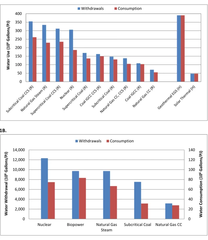
Water factors from the NREL study were converted into units of millions of gallons
consumed and withdrawn per petajoule (PJ) of electricity output for each
electricity-generating technology. These water factors are displayed in Figure 1 for technologies
operating recirculating, hybrid and once-through cooling systems. In general, water factors
decrease for plants with greater generation efficiency. Based on analysis by the U.S.
Department of Energy, it was assumed that all electric generating plants built in the future
will install recirculating cooling systems.23
It was also assumed that wind turbines neither withdraw nor consume any water,
12
hydropower based on increased evaporation from reservoirs.20,7 However, we defined no
water withdrawal or consumption for hydroelectric power generation because the
evaporative losses resulting from hydropower reservoirs can also be attributed to other
purposes such as water supply, flood control and recreation. This study only analyzes the
quantity of water used during the process of electricity generation. As such, water used by
other sectors and processes such as resource extraction are not reported here. Effects on
water quality are also not addressed in this study.
To determine the total once-through and recirculating cooling capacities currently
installed on existing thermoelectric power plants, we aggregated power plant survey data
from the DOE’s Energy Information Administration (EIA). We compiled cooling system data
from 2005 EIA Form 767 as well as 2006-2011 EIA Form 860reports. 26,27 In some cases,
cooling system entries differed between years for the same unit. Wherever cooling system
entries from two survey years conflicted, the later entry was used. These survey datasets
provided cooling system codes for the units on many existing natural gas and coal-fired
thermoelectric power plants. However, these forms do not collect data on nuclear power
plants. In addition, many of the power plants surveyed omitted the cooling system entry on
the survey response. This resulted in significant gaps in the aggregated dataset including no
cooling data on 128 of 600 coal plants, 558 of 5,094 natural gas plants and all 104 nuclear
power plants.
To complete this dataset, power plants with cooling systems unaccounted for in EIA
datasets were individually identified and coded by visual identification with satellite
13
Facility Locator.16 Latitude and longitude data for coal-fired power plants and some natural
gas facilities were identified with the Center for Media and Democracy’s Sourcewatch3.
Using location data, satellite images of each power plant were examined with Bing and
Google maps and compared to known photographs of the plant. Through identification of
definitive cooling systems features such as cooling towers and ponds, each plant cooling
system was coded. 131 natural gas power plants could not be located and were assumed to
14 1A.
1B.
Figure 1. Water Withdrawal and Consumption Factors. Water withdrawal and consumption factors for all modeled technologies using recirculating (R) and hybrid (H) cooling systems (1A) and for once-through cooling (1B). Technology acronyms: CC = combined cycle, IGCC = integrated gasification combined cycle, CCS = carbon capture and storage, EGS = enhanced geothermal system.
0 50 100 150 200 250 300 350 400 W a te r U se ( 1 0 6G a ll o n s/ P J) Withdrawals Consumption 0 20 40 60 80 100 120 140 0 2,000 4,000 6,000 8,000 10,000 12,000 14,000
Nuclear Biopower Natural Gas Steam
Subcritical Coal Natural Gas CC
IV.
Results
We first present changes in the total energy system response to CO2 constraints,
then changes within the electric sector, and finally implications of those changes for electric
sector water withdrawal and consumption.
Model Response to Constraints by Sector
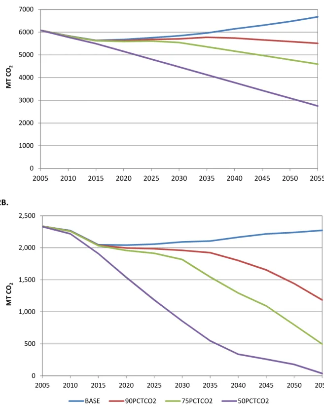
Total U.S. energy system CO2 emissions and electric sector CO2 emissions from 2005
to 2055 for all four policy scenarios are shown in Figures 2A and 2B respectively. Model
results under all scenarios show an initial decrease in both total system and electric sector
CO2 emissions between 2005 and 2015 in response to a drop in energy demand during that
period due to economic conditions.28 In the Base scenario, total system and electric sector
CO2 emissions gradually increase from 2015 through the model time horizon as demand for
energy services continues to increase. By 2055, total system CO2 emissions exceed 2005
values by 10%. CO2 emissions from the electric sector in 2055 remain slightly below 2005
values in spite of increased demand as a result of increased electric generating efficiency.
In both the 10% and 25% CO2 Reduction scenarios, electric sector emissions actually
decrease more than total energy system CO2 emissions over the model horizon because
other sectors (such as transportation) continue to grow in CO2 emissions during that time.
This discrepancy between the CO2 emissions reduction shares of different sectors illustrates
16
sectors. As a result, the model maximizes electric sector emissions reductions before it
becomes economically viable to make changes in other sectors.
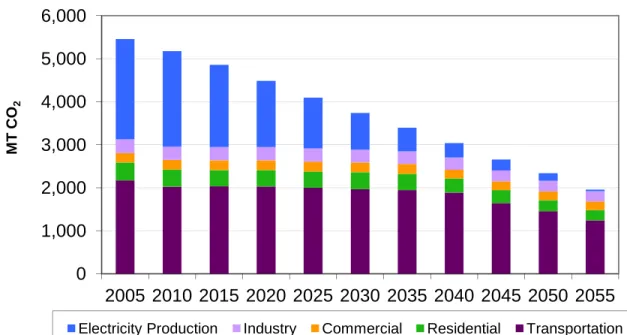
Under the 50% CO2 Reduction scenario, electric sector CO2 emissions drop to nearly
zero by 2055. Total energy system CO2 emissions decrease by 3,327 Mt/yr in 2055. Of
these reductions, only 60% comes from the electric sector (1,996 Mt) and 30% comes from
the transportation sector (998 Mt). The remaining decreases come from the industrial,
residential and commercial sectors. CO2 emissions by sector from 2005 to 2055 under the
50% CO2 Reduction scenario are shown in Figure 3A.
Changes in transportation sector emissions first take on a significant share of total
system emissions reductions in 2045, once electric sector emissions have already decreased
to nearly 10% of their 2005 value. Transportation sector emissions reductions are achieved
primarily through changes in light duty vehicles. Differences in light duty vehicle technology
use between the base and the 50% CO2 Reduction scenarios are shown in Figure 3B.
Emission reductions by the light duty vehicle sector are achieved through increased use of
ethanol (E85) in vehicles operating internal combustion engines as well as plug-in hybrids.
Electric vehicles and vehicles running on compressed natural gas also play a role in reducing
light duty vehicle emissions.
The substantial increase in the use of both electric vehicles and plug-in hybrids after
2045 under the 50% CO2 Reduction scenario means that the total demand for electricity by
the light duty vehicle sector increases dramatically. This increased use of electricity by the
transportation sector requires a corresponding increase in total electricity production in the
17 2A.
2B.
Figure 2. System and Sector CO2 Emissions. U.S energy system CO2 emissions for all scenarios (2A). Electric sector CO2 emissions for all scenarios (2B).
0 1000 2000 3000 4000 5000 6000 7000
2005 2010 2015 2020 2025 2030 2035 2040 2045 2050 2055
M
T
C
O2
0 500 1,000 1,500 2,000 2,500
2005 2010 2015 2020 2025 2030 2035 2040 2045 2050 2055
M
T
C
O2
18 3A.
3B.
Figure 3. CO2 Emissions by Sector and Light Duty Vehicle Technologies. CO2 emissions from end-use sectors in the 50% CO2 Reduction scenario (3A). Differences in light duty vehicle technologies between the Base and 50% CO2 Reduction scenarios (3B). Positive values indicate technologies used more in the 50% CO2 Reduction scenario and negative values indicate technologies used more in the Base scenario. Figure legend abbreviations: CNG = compressed natural gas, ICE = internal combustion engine, E85 = 85% ethanol fuel blend, GSL = gasoline. Plug-in X, where X refers to the vehicles electric range in miles.
0 1,000 2,000 3,000 4,000 5,000 6,000
2005 2010 2015 2020 2025 2030 2035 2040 2045 2050 2055
M
T
C
O2
Electricity Production Industry Commercial Residential Transportation
-4 -3 -2 -1 0 1 2 3 4
2005 2010 2015 2020 2025 2030 2035 2040 2045 2050 2055
T ri li o n V e h ic le M il e s T ra v e ll e d P e r Y e a
r Electric Vehicles
19 Electric Sector Technology Changes
Electric sector technology use in each modeled scenario is shown in Figure 4. Under
the 10% CO2 Reduction scenario (Figure 4B), most conventional coal-fired power plants that
remained active to 2055 under the base scenario are gradually taken out of use. The
majority of the conventional coal facilities that are not retired are retrofitted with carbon
capture and storage (CCS) technology. In place of the coal facilities that were taken offline,
the model significantly increases power generation by natural gas combined cycle power
plants and wind power.
In the 25% CO2 Reduction scenario, conventional coal plants are retired more rapidly
and are taken completely out of use by 2050. The model continues to rely primarily on
natural gas combined cycle and wind to replace these decreases in coal use. In 2040, solar
thermal power production is also implemented to contribute a significant share of total
electricity generation, and its use increases throughout the remaining years. In 2055,
natural gas combined cycle with CCS replaces over 30% of existing natural gas power
generation.
In the 50% CO2 Reduction scenario, the significant increase in electricity demand
from light duty vehicle electrification leads to large increases in total electricity generation
after 2035 (33% greater in 2055 than in the base case). At the same time, total electric
sector CO2 emissions approach zero (Figure 1B). To simultaneously increase electricity
generation and decrease emissions by such substantial margins requires great changes in
electric sector technology mix. Conventional coal-fired power plants are taken completely
20
existing natural gas and grows to generate 8513 PJ by 2055. Total U.S. carbon storage
capacity is represented in the model, but does not impact the CCS use because the storage
capacity is so great.15 Use of renewable power, including wind, solar, and hydropower, also
21 4A. 4B. -5,000 10,000 15,000 20,000 25,000 30,000
2005 2010 2015 2020 2025 2030 2035 2040 2045 2050 2055
Q u a n ti ty ( P J /y r) Base -5,000 10,000 15,000 20,000 25,000 30,000
2005 2010 2015 2020 2025 2030 2035 2040 2045 2050 2055
Q u a n ti ty ( P J /y r)
10% CO2Reduction
Distributed Solar PV Central Solar PV Central Solar Thermal Wind Power
Hydropower Geothermal Power
Municipal Waste to Steam Biomass to IGCC
Conventional Nuclear Power Residual Fuel Oil to Steam Diesel to Combined Cycle Diesel to Combustion Turbine NGA to Combined-Cycle-CCS NGA to Combined-Cycle NGA to Combustion Turbine NGA to Steam Electric Coal to Steam-CCS Retro Coal to Steam
22 4C.
4D.
Figures 4. Electric Sector Technology Mix. Electricity production by technology for each scenario from 2005 to 2055.
-5,000 10,000 15,000 20,000 25,000 30,000
2005 2010 2015 2020 2025 2030 2035 2040 2045 2050 2055
Q u a n ti ty ( P J /y r)
25% CO2Reduction
-5,000 10,000 15,000 20,000 25,000 30,000
2005 2010 2015 2020 2025 2030 2035 2040 2045 2050 2055
Q u a n ti ty ( P J /y r)
50% CO2Reduction
Distributed Solar PV Central Solar PV Central Solar Thermal Wind Power
Hydropower Geothermal Power
Municipal Waste to Steam Biomass to IGCC
Conventional Nuclear Power Residual Fuel Oil to Steam Diesel to Combined Cycle Diesel to Combustion Turbine NGA to Combined-Cycle-CCS NGA to Combined-Cycle NGA to Combustion Turbine NGA to Steam Electric Coal to Steam-CCS Retro Coal to Steam
23 Electric Sector Technology Changes by Region
The electric sector technology mix for each region under the Base and 50% CO2
Reduction scenarios for 2055 is shown in Figure 5. The electric sector response to CO2
emissions constraints varies considerably between regions. In eastern regions (1, 2, 3, 5,
and 6), use of nuclear power and natural gas combined cycle with CCS increases
dramatically by 2055 under the 50% CO2 Reduction scenario. In contrast, central and
western regions (4, 7 and 8) expand electricity-generating capacity primarily with wind
power. Regions 9 and 7 also incorporate significant generating capacity from concentrated
solar thermal as well as natural gas combined cycle with CCS.
One of the primary drivers for these differences in technology choices between
regions is resource availability. In eastern regions, renewable resource availability (such as
for wind, solar or geothermal power generation) is relatively poor.6,24,28 Technology choices
in eastern regions are therefore restricted to rely primarily on non-renewable low-carbon
technologies, such as nuclear and natural gas with CCS, to satisfy CO2 constraints. In
contrast, western regions have favorable renewable resource availability, making the
implementation of wind and solar power far more attractive in those regions.6,24,28
Another significant determinant of the electricity generation technology differences
between regions is the projected vehicle-miles-traveled (VMT) in each region. Region 5 is
projected to see the greatest expansion in total VMT’s of any region over the modeled time
horizon. This has several effects on the model results. First, as a result of these increases,
region 5 shows the largest increase in total electricity production from the base to the 50%
24
implementation of nuclear power in region 5 under the 50% CO2 Reduction scenario.
Electric vehicles and plug-in hybrids are typically charged at night and thus have the effect
of increasing base load demand and decreasing fluctuations in demand for electricity. This
increase in base load electricity demand makes nuclear power production in that region
more favorable.
In contrast, lower projected growth in population and VMT in mountain western
regions mean that implementation of renewable energy technologies (particularly wind)
can be used to supplement electricity in other regions when it is available. Total
interregional transfers increase by almost 40% from the Base to the 50% CO2 Reduction
Scenario (Figure 6). Under the 50% CO2 Reduction scenario, regions 4, 7, and 8 use their
substantial renewable energy resources to supply low carbon electricity to other regions
through trading. These regions export 28%, 9% and 17% of their total electricity production
respectively in 2055. To accommodate these substantial exports, regions 4 and 8 undergo
the largest increase in total electricity generation by percentage of any region, as they
increase by 75% and 98% in total electricity generation respectively.
All other regions become net importers, with the most substantial imports going to
regions 5 and 6. Though region 5 remains one of the largest importers nationally, its share
of total electricity imports decreases from the Base to the 50% CO2 Reduction scenario
because of its substantial increase in nuclear base load capacity. All regions except for
region 6 also increase total electricity generation from the Base to the 50% CO2 Reduction
scenario in 2055 to accommodate the increased demand for electricity from electric and
25
reliance on imported electricity in region 6 is likely the product of low renewable energy
availability in that region paired with immediate proximity to regions with vastly greater
renewable energy potential (regions 4 and 7), making it particularly cost-effective to import
2
6
Figure 5. Electric Sector Technology Mix by Region. Electricity production (PJ) by technology in the Base (left bar) and the 50%
CO2 Reduction scenarios (right bar) in 2055 in nine regions.
Distributed Solar PV Central Solar PV Central Solar Thermal Wind Power
Hydropower Geothermal Power Municipal Waste to Steam Biomass to IGCC
6A.
6B.
Figures 6. Net Flows of Electricity.
scenario (6A) and 50% CO2 emissions reduction scenario proportional to the quantity of electricity traded.
27
Net Flows of Electricity. Net flows of electricity between regions under the emissions reduction scenario (6B) in 2055. Arrow width is proportional to the quantity of electricity traded.
28 Electric Sector Water Use
Total electric sector water withdrawal and consumption for all four scenarios are
shown in Figure 7. This figure shows that electric sector water withdrawal is strongly
influenced by CO2 constraints; as CO2 emissions decrease, water withdrawal decreases as
well. In the 50% CO2 Reduction scenario, total electric sector water withdrawal decreases to
less than 45% of 2005 values by 2035. This considerable reduction in water withdrawal
results from several factors. First, as existing once-through capacity is replaced with newer
technologies, our assumption that all new power plants will be built with recirculating
cooling systems causes water withdrawal to decrease substantially. Second, a large share of
total electricity generation is shifted to lower-water use renewable power sources (wind
and solar). Finally, replacement of old power generating facilities with newer technologies
mean total electric generating efficiency increases over the model horizon, thereby
decreasing water withdrawal.
The response of electric sector water consumption is more complex. Under the
Base scenario, water consumption increases over the model time horizon as a result of
increased electricity production and because existing power plants with once-through
cooling systems are gradually replaced by plants with recirculating cooling systems, for
which water withdrawal is less but consumption is greater. Under all three CO2 constraint
scenarios, there is a period in which total electric sector water consumption decreases as
the CO2 emissions constraints force the model to retire conventional coal-fired power plants
and replace them with more efficient natural gas combined cycle plants. These decreases
29
plant retirement. For the 10%, 25%, and 50% CO2 Reduction scenarios, the lowest
consumption occurs in 2050, 2040, and 2030 respectively.
After this initial decrease, water consumption in each scenario then begins to
increase again as new coal and natural gas CCS plants are brought online. CCS technology
consumes large quantities of water because of the considerable parasitic load it imposes on
its generator and because the amine scrubbing process modeled here is highly water
intensive.12 Under the 50% CO2 Reduction scenario, water consumption increases by over
60% from 2005 values by 2055. This considerable jump in water consumption is largely a
product of the increased use of natural gas combined cycle with CCS as well as the faster
transition to recirculating cooling.
Each CO2 emissions constraint scenario has a unique impact on total electric sector
water consumption. In the 10% CO2 Reduction scenario, electric sector water consumption
is less than base case consumption throughout the model horizon because of the
substantial conventional coal plant retirement and small CCS penetration. In the 25% CO2
Reduction scenario, electric sector water consumption remains significantly below base case
values until the last model time step when CCS implementation begins to take on a more
substantial share of total electricity production. Finally, under the 50% CO2 Reduction
scenario, water consumption increases 40% over base case values by 2055. This
considerable jump in water consumption is largely a product of the considerable use of
natural gas combined cycle with CCS as well as the faster transition to recirculating cooling.
Regional shares of total electric sector water withdrawal and consumption are
30
relatively static throughout the time horizon in the base case. As CO2 constraints take
effect, regional shares of both total electric sector water withdrawal and consumption begin
to change. In the 50% CO2 Reduction scenario, regions 4, 6, 7 and 8 show significant
decreases in overall water withdrawal. This results from the decrease in total electricity
output (region 6) and the considerable increase in wind-powered electricity generation in
those regions (regions 4, 7 and 8). For the same scenario, regions 3 and 5 make significant
increases in total electric sector water consumption. These changes reflect major increases
in the use of nuclear power and natural gas with CCS electricity generating technologies as
31 7A.
7B.
Figure 7. Electric Sector Water Use. Electric sector water withdrawal (7A) and consumption (7B). 15 20 25 30 35 40 45
2005 2010 2015 2020 2025 2030 2035 2040 2045 2050 2055
W it h d ra w a l (1 0 1 2G a ll o n s/ y r) 1.0 1.2 1.4 1.6 1.8 2.0
2005 2010 2015 2020 2025 2030 2035 2040 2045 2050 2055
Withdrawal (10 B a se 5 0 % C O2 R e d u ct io n
Figure 8. Electric sector water withdrawal and consumption by region 0 5 10 15 20 25 30 35 40 45 50
2005 2010 2015 2020 2025 2030 2035
0 5 10 15 20 25 30 35 40 45 50
2005 2010 2015 2020 2025 2030 2035
R1
32
(1012 gal/yr) Consumption (10
Electric sector water withdrawal and consumption by region
50% CO2 Reduction scenarios.
2035 2040 2045 2050 2055
0 0.2 0.4 0.6 0.8 1 1.2 1.4 1.6 1.8 2
2005 2010 2015 2020 2025 2030 2035
2035 2040 2045 2050 2055
0 0.2 0.4 0.6 0.8 1 1.2 1.4 1.6 1.8 2
2005 2010 2015 2020 2025 2030 2035
R2
R3
R4
R5
R6
R7
R8
(1012 gal/yr)
Electric sector water withdrawal and consumption by region for the Base and
2035 2040 2045 2050 2055
2035 2040 2045 2050 2055
V.
Sensitivity Analysis
Three technologies dominated the electric sector under the 50% CO2 Reduction
scenario: natural gas with CCS, nuclear, and wind. Here we test the sensitivity of the results
of this scenario to incentives and restrictions on these three technologies. We focus our
comparison on results in the end-year of the model: 2055.
Scenarios
We conducted nine sensitivity analysis scenarios. Each scenario incorporates a
change to a single technology while maintaining the 50% CO2 emissions reduction
constraint. In the CCS Cost Down scenario, the investment costs for all CCS technologies
were reduced 50% in each year of the model time horizon relative to their cost under the
50% CO2 Reduction scenario. The CCS Cost Up scenario increases them 50%. The No CCS
scenario restricts the model from using any CCS to meet electricity demand, either through
retrofits or through construction of new plants.
In the No Nuclear Constraint scenario, constraints on nuclear power that exist under
base case conditions were removed. These constraints are based on AEO 2012 projections,
and do not impact system results in the Base scenario, but restrict total nuclear power
under the 50% CO2 Reduction scenario. In the Nuclear Cost Up scenario, the investment
cost for new nuclear power plants is increased 50% in all model years relative to the cost
34 from building any new nuclear capacity entirely.
The Wind Cost Down and Wind Cost Up scenarios reduced and increased
respectively the investment cost for all wind technology by 50% relative to the costs under
the 50% CO2 Reduction scenario in all modeled years. Finally, the Reduced Wind scenario
restricts electricity generation from wind to half of that generated under the 50% CO2
Reduction scenario in year 2055 for regions 4, 7, and 8 throughout the model time horizon.
Wind power in all other regions was not restricted in this scenario because wind did not
serve as a primary source of electricity generation in those regions under the 50% CO2
Reduction scenario.
Results
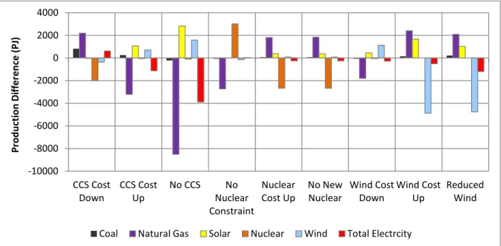
Net changes in electricity generation from five major energy sources (coal, natural
gas, solar, nuclear and wind) relative to the 50% CO2 Reduction scenario under each
sensitivity analysis scenario are shown in Figure 9A. Net changes in total water withdrawal
and consumption for each scenario are shown in Figure 9B. For comparison, total national
electricity generation in 2055 under the 50% CO2 Reduction scenario was 26,136 PJ while
national water withdrawal was 19.4 trillion gallons and water consumption was 1.9 trillion
gallons.
The model responded to the CCS Cost Down scenario with increased use of natural
gas CCS and coal CCS and decreased use of nuclear power and wind. Total electricity
generation increased slightly in response to this decrease in cost. These changes led to a
35
decreased nuclear power (2% and 1% respectively relative to the 50% CO2 Reduction
scenario national total).
The CCS Cost Up scenario caused a 3221 PJ decrease in electricity generation from
natural gas, but a 610 PJ increase in the use of CCS retrofits to existing coal capacity, even
though the investment cost for those retrofits were also increased in that scenario. This
occurred because the coal CCS retrofits were the cheapest CCS option available to the
model. In place of the natural gas, the model used increased wind and solar. Overall, these
changes resulted in an over 1100 PJ decrease in total electricity generation. Water
withdrawal increased substantially (0.37 trillion gallons) as a result of the continued use of
existing coal facilities with open loop cooling systems. Water consumption, however,
decreased as the overall use of CCS technology was significantly reduced from the 50% CO2
Reduction scenario.
The No CCS scenario produced the most drastic changes in technology mix and total
electricity generation. Total electricity generation decreased 3,881 PJ from the 50% CO2
Reduction scenario – nearly 15% with respect to the 50% CO2 Reduction scenario. This
reduction in total electricity generation was accommodated by reductions in transportation
sector electricity use. In response to the increased price of electricity, the model used
fewer electric vehicles and, in their place, used more vehicles running on biofuels and
compressed natural gas.
Changes in technology mix included an over 8000 PJ decrease in the use of natural
gas and coal (nearly all of what was used under the 50% CO2 Reduction scenario), and an
36
changes led to a 1.74 trillion gallon decrease in electric sector water withdrawal (8.9% of
the national total in the 50% CO2 Reduction scenario) and a 0.9 trillion gallon decrease in
electric sector water consumption (45% of the national total in the 50% CO2 Reduction
scenario).
In the No Nuclear Constraint scenario, 3022 PJ more nuclear power was used to
meet electricity demand than had been used in the 50% CO2 Reduction scenario. This
increase in nuclear power primarily replaced natural gas combined cycle with CCS and led to
increases in both water withdrawal and consumption. Impact on coal, solar, wind and total
electricity generation was negligible. The Nuclear Cost Up and the No New Nuclear scenario
produced almost identical results. Nuclear electricity generation decreased 2670 PJ and
was replaced by an 1811 PJ increase in the use of natural gas combined cycle with CCS.
Both scenarios led to a small decrease in total electricity generation (254 PJ). Both
scenarios produced moderate decreases in water withdrawal (0.45 trillion gallons, 2% of the
national total in the 50% CO2 Reduction scenario) and consumption (0.28 trillion gallons,
14% of the national total in the 50% CO2 Reduction scenario).
The Wind Cost Down scenario led to increased use of wind power in place of natural
gas combined cycle with CCS. These changes resulted in the second largest decrease in
water withdrawal at 0.69 trillion gallons of water (4% relative to the 50% CO2 Reduction
scenario national total). Finally, the Wind Cost Up and the Reduced Wind scenarios led to
similar, but not identical results. Both included an overall decrease in electricity generation
(3% and 4% respectively relative to the 50% CO2 Reduction scenario national total). These
37
compressed natural gas vehicle use. Total electricity generation from wind power
decreased 4877 PJ and 4758 PJ respectively (roughly 18% of the national total in the 50%
CO2 Reduction scenario) but was partially compensated for by increased use of natural gas
with CCS, solar and coal with CCS in both scenarios. These changes led to the largest
increases in electric sector water withdrawal and consumption at roughly 4% of the total
national water withdrawal and 15% of the national water consumption in the 50% CO2
Reduction scenario.
Implications
One of the most noteworthy takeaways of these scenarios is that changes in the
availability or cost of a single electric sector technology can have major impacts on the
transportation sector technology portfolio. In almost all the scenarios modeled, impacts on
total electricity generation were paired with changes to electric transportation sector
technologies such as the decrease in the use of electric vehicles and plug-in hybrids
combined with an increase in the use of compressed natural gas vehicles and vehicles
running on biofuels.
The CCS Cost Up scenario was the only one to cause an increase in total electric
sector water withdrawal and a decrease in water consumption. All other scenarios
produced changes in electric sector water withdrawal and consumption of the same sign
(either negative or positive). Predictably, scenarios causing decreased use of wind (Wind
Cost Up and Reduced Wind) were the scenarios causing the most substantial increase in
national water withdrawal and consumption. The No CCS scenario, however, was the
38 9A.
9B.
Figure 9. Sensitivity Analysis. Difference in electricity generation in 2055 between the 50% CO2
Reduction Scenario and six sensitivity analysis scenarios for five major energy source categories (PJ) (9A). Difference in annual water withdrawal and consumption in year 2055 between the 50% CO2
Reduction scenario and six sensitivity analysis scenarios (9B). Percent change from the 2055 50%
CO2 Reduction scenario withdrawal and consumption are displayed next to each scenario.
-10000 -8000 -6000 -4000 -2000 0 2000 4000 CCS Cost Down CCS Cost Up
No CCS No Nuclear Constraint Nuclear Cost Up No New Nuclear Wind Cost Down Wind Cost Up Reduced Wind P ro d u ct io n D if fe re n ce ( P J)
Coal Natural Gas Solar Nuclear Wind Total Electrcity
-2 -1.5 -1 -0.5 0 0.5 1 CCS Cost Down CCS Cost Up
No CCS No Nuclear Constraint Nuclear Cost Up No New Nuclear Wind Cost Down Wind Cost Up Reduced Wind C h a n g e i n W a te r U se ( 1 0 1 2G a ll o n s/ y r)
VI.
Conclusions
Constraints on U.S. energy system CO2 emissions could have significant impacts on
the water use of the electric sector. The model responded to CO2 emissions constraints
with electric sector technology changes that led to decreased overall water withdrawal in all
scenarios. These changes also decreased water consumption under the 10% CO2 Reduction
scenario, but led to an overall increase in water consumption under the 25% and 50% CO2
Reduction scenarios in 2055. These changes in technology mix included decreased use of
conventional coal and natural gas powered electricity generation and increased use of
renewable technologies such as wind and solar, as well as nuclear power and natural gas
combined cycle with CCS. In the 50% CO2 Reduction scenario, these changes were also
driven by increased demand for electricity from the transportation sector resulting from
vehicle electrification.
These technology changes and the associated decrease in total electric sector water
withdrawal could significantly reduce aggregate national electric sector vulnerability to
climate change. The decrease in total system water withdrawal that resulted under the CO2
emission constraint scenarios reduces the potential for low stream flows and high water
temperatures to impact electricity generating capacity. Moreover, the technology changes
associated with these CO2 constraints accelerated the switch from once-through cooling
40
cooling systems do not require the discharge of heated water back into ambient water
bodies and thus are not susceptible to water-quality regulations that may prohibit cooling
on hot days.
The increased aggregate national water consumption of the electric sector under
CO2 emissions constraints is less likely to impact electric sector vulnerability to climate
change than is water withdrawal, but it could lead to different negative impacts. The
electric sector currently accounts for only 6% of national water consumption, but that value
is projected to almost double by 2055 in the 50% CO2 Reduction scenario.1 As electric
sector water consumption increases, competition with other water users such as agriculture
and municipalities could lead to localized cooling water shortages and in extreme
conditions, potentially result in localized electric power failures.
To interpret these results on a regional level, it will be critical to understand where
climate change impacts on water resources are expected to occur. Previous regional
analyses of future climate change impacts on water resources in the United States project
that the most severe changes in water temperature highs and stream-flow lows will occur in
south-central, south-eastern and mid-western states.17,30 Our model results in western
regions (regions 4, 7, 8 and 9) incorporated large wind power capacity under CO2
constraints (especially 4 and 8) as well as solar thermal power (regions 7 and 9). These
changes had the effect of driving both water withdrawal and water consumption down
significantly in those regions, making them more resilient to variability in water resources
41
region 7, which includes Texas and Oklahoma, where regional projections of decreased
precipitation and increased water temperature are some of the most severe nationally.17,30
In contrast, eastern regions (regions 1, 2, 3, 5 and 6) met electricity demand
primarily through nuclear power (most notably in region 5) and natural gas combined cycle
with CCS (regions 2 and 3). As a result, water withdrawal decreased less in these regions
relative to the national average, but water consumption rose dramatically in the 50% CO2
Reduction scenario. These changes would have the overall effect of decreasing electric
sector vulnerability to changes in water resource availability in eastern regions. However, in
light of the substantial projected climate change impacts on water resources in these
regions (particularly in regions 3, 5, and 6), electric power reliability may still be threatened
by climate change even under this most extreme CO2 constraint scenario. Of these regions,
region 5 would likely be the most vulnerable because of its heavy use of nuclear power and
its associated water withdrawal.
In conclusion, these findings suggest that U.S. energy policies aimed at reducing
total CO2 emissions are likely to have complex impacts on the electric sector. The overall
reduction in electric sector water withdrawal and increased penetration of low water-use
technologies, such as wind and solar power, are likely to reduce electric sector vulnerability
to climate change. However, in eastern regions where electric sector changes would be
likely to incorporate higher water-use technologies, these benefits will be less significant. In
addition, the increased water consumption resulting from the shift to recirculating cooling
systems may lead to issues with electric power reliability as a result of competition with
42
These conclusions must be considered in the context of the uncertainties and
limitations inherent to the model and data sources. First, as an optimization model,
MARKAL cannot predict how the U.S. energy system would develop under any policy
scenario. Instead, MARKAL prescribes the most cost-effective system-wide solution based
on the inputs it is given. As such, our results do not account for un-modeled factors such as
consumer behavior, public opinion, and politics. These factors will likely have significant
impacts on future energy choices that we cannot anticipate, especially for energy sources
such as wind and nuclear power.
Second, there is uncertainty in the data used for this analysis. Model results are
informed by AEO 2012 projections of demands, costs and available technologies. Although
near term demands and technologies are relatively well characterized, the medium and
long-term values are more uncertain. Future changes in the costs and efficiency of existing
technologies, or the invention of new “breakthrough” technologies, could have dramatic
effects on the energy choices the model makes as well as on the water use associated with
those energy choices. Furthermore, AEO 2012 only provides projections on these variables
out to 2035. As a result, 20 years of data are based on extrapolation of AEO forecasts for
these variables.
Future extensions of this work could evaluate how alternative energy system
responses to the same CO2 constraints could impact electric sector water use. Possible
alternative energy system responses could incorporate greater use of nuclear power, CCS or
renewables relative to our current model results. In addition, future work could explore in
Appendix A
10A.10B.
Figure 10. Water withdrawal in trillions of gallons for each region in 2055 for the bar) and the 50% CO2 Reduction
gallons for each region in 2055 for the (right bar)(10B).
43
Appendix A: Regional Water Use
Water withdrawal in trillions of gallons for each region in 2055 for the
eduction scenarios (right bar) (10A).Water consumption
gallons for each region in 2055 for the Base (left bar) and the 50% CO2 Reduction
Water withdrawal in trillions of gallons for each region in 2055 for the Base (left consumption in trillions of
Appendix B
11A.11B.
Figure 11. Net interregional flows of embodied water consumption (billion gallons/yr) in the Base scenario (11A). Net interregional flows of embodied water consumption (billion gallons/yr) in the 50% CO2 Reduction
44
Appendix B: Net Flows of Embodied Water
Net interregional flows of embodied water consumption (billion gallons/yr) in Net interregional flows of embodied water consumption (billion
eduction scenario (11B). Arrow sizes correspond to size of flow.
Net interregional flows of embodied water consumption (billion gallons/yr) in Net interregional flows of embodied water consumption (billion
45
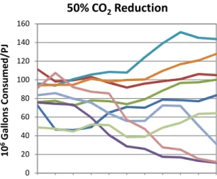
Appendix C: Water Use vs. Electricity Use by Region
12A. 12B.
12C. 12D.
Figure 12. Water consumption per unit electricity generated (million gallons /PJ) for each region in the Base scenario (12A) and the 50% CO2 Reduction scenario (12B). Water withdrawal per unit electricity generated (billion gallons/PJ) for each region in the Base scenario (12C) and the 50% CO2 Reduction scenario (12D).
0 20 40 60 80 100 120
2005 2010 2015 2020 2025 2030 2035 2040 2045 2050 2055
1 0 6G a ll o n s C o n su m e d /P J Base 0 20 40 60 80 100 120 140 160
2005 2010 2015 2020 2025 2030 2035 2040 2045 2050 2055
1 0 6G a ll o n s C o n su m e d /P J
50% CO2Reduction
0 1 2 3 4 5 6
2005 2015 2025 2035 2045 2055
1 0 6G a ll o n s W it h d ra w n /P J Base 0 1 2 3 4 5 6
2005 2015 2025 2035 2045 2055
1 0 6G a ll o n s W it h d ra w n /P J
46
Works Cited
1. Carter, N. T. Energy’s Water Demand: Trends, Vulnerabilities, and Management. Congressional Research Service. 2010, R41507.
2. California Energy Commission. Comparison of Alternate Cooling
Technologies for California Power Plants: Economic, Environmental and Other Tradeoffs. Public Interest Energy Research, 2002, 500-02-079F.
3. Center for Media and Democracy. Sourcewatch. Retrieved on 11-12-2012 from:
www.sourcewatch.org/index.php/Portal:Coal_Issues
4. Dodder, R.; Yelverton, W.; Felgenhauer, T.; King, C. Water and greenhouse gas tradeoffs associated with a transition to a low carbon transportation system.
International Mechanical Engineering Congress and Exposition, 2011, Denver,
Colorado.
5. Eilperin, J. Drought puts squeeze on hydroelectric grid. Seattle Times, September 22, 2012.
6. Elliot, D.L., Wendell, L.L., Glower, G.L. An Assessment of the Available Windy Land Area and Wind Energy Potential in the Contiguous United States. Department of Energy, Pacific Northwest Laboratory. 1991, PNL-7789.
7. Gleick, P. Environmental Consequences of Hydroelectric Development: The Role of Facility Size and Type. Energy. 1992, Vol. 17 (8), pp. 735–747.
8. Kenny, J.F., Barber, N.L., Hutson, S.S., Linsey, K.S., Lovelace, J.K., and Maupin, M.A. Estimated use of water in the United States in 2005: U.S. Geological Survey Circular. 2009, 1344, 52 p.
9. Kimmel, T. and Veil, J. Impact of Drought on U.S. Steam Electric Power Plant Cooling Water Intakes and Related Water Resource Management Issues. National Energy Technology Laboratory, Department of Energy. 2009, DOE/NETL-2009/1364.
10.Library of Congress, Bill Summary and Status, 111th Congress (2009 - 2010), H.R.2454. Retrieved on 11-9-2012 from:
thomas.loc.gov/cgi-bin/bdquery/z?d111:H.R.2454.
47
12.Macknick, J., R. Newmark, G. Heath, and K.C. Hallet. A Review of Operational Water Consumption and Withdrawal Factors for Electricity Generating Technologies. National Renewable Energy Laboratory. 2011, NREL/TP-6A20-50900.
13.Macknick, J. R.; Sattler, S.; Averyt, K.; Clemmer, S.; and Rogers, J. The water
implications of generating electricity: water use across the United States based on different electricity pathways through 2050. Environmental Research Letters. 2012, Vol. 7, No. 4, doi:10.1088/1748-9326/7/4/045803.
14.MSNBC. U.S. sets climate target ahead of summit. Retrieved on 11-29-2012 from:
http://www.msnbc.msn.com/id/34147586/ns/us_news-environment/t/us-sets-climate-target-ahead-summit/#.ULe9LWeCf38”
15.National Energy Technology Laboratory. Carbon Sequestration Atlas of the Untied States and Canada. 2010, Third Edition, Atlas 3. Retreived on 2-20-2013 from:
http://www.netl.doe.gov/technologies/carbon_seq/refshelf/atlas/.
16.Nuclear Regulatory Commission FacilityLocator, retrieved on 11-9-2012 from
http://www.nrc.gov/info-finder/reactor/.
17.Roy S. B.; Chen, L.; Girvetz, E. H.; Maurer, E. P.; Mills, W. B.; and Grieb, T. M. Projecting Water Withdrawal and Supply for Future Decades in the U.S. under Climate Change Scenarios. Environmental Science & Technology. 2012, 46 (5), 2545-2556.
18.Shay, C. L. and Loughlin, D. H. Development of a Regional U.S. MARKAL Database for Energy and Emissions Modeling. In Global Energy Systems and Common
Analyses--Final Report of Annex X (2005-2008); Goldstein, G. and Tosato, G.; International
Energy Agency, Paris, France 2008: pp. 123-125.
19.Shay, C.; Dodder, R.; Gage, C.; Kaplan, O.; Loughlin, D.; Yelverton, W. EPA U.S. Nine Region MARKAL Database, Database Documentation. Air Pollution Prevention and Control Division, National Risk Management Research Laboratory, U.S.
Environmental Protection Agency. 2012.
20.Torcellini, P., Long, N., Judkoff, R. Consumptive Water Use for U.S. Power Production. National Renewable Energy Laboratory. 2003.
21.Union of Concerned Scientists. Rising Temperatures Undermine Nuclear Power's Promise,” Union of Concerned Scientists. 2007.