Savascin_unc_0153D_12954.pdf

ENDOGENOUSLY CLUSTERED FACTOR APPROACH TO MACROECONOMICS

OZGE SAVASCIN

A dissertation submitted to the faculty of the University of North Carolina at Chapel Hill in

partial ful…llment of the requirements for the degree of Doctor of Philosophy in the Department

of Economics.

Chapel Hill

2012

ABSTRACT

OZGE SAVASCIN: Endogenously Clustered Factor Approach to Macroeconomics

(Under the direction of Neville R. Francis)

This dissertation constructs a novel factor approach to study the comovements of

macro-economic variables and introduces its two practical applications.

Factor models have become useful tools for studying international business cycles.

Block factor models can be especially useful as the zero restrictions on the loadings of some

fac-tors may provide some economic interpretation of the facfac-tors. These models, however, require

the econometrician to prede…ne the blocks, leading to potential misspeci…cation. In my

coau-thored paper, we propose an alternative model in which the blocks are chosen endogenously.

The model is estimated in a Bayesian framework using a hierarchical prior which allows

series-level covariates to in‡uence and explain how the series are grouped. Using similar international

business cycle data as Kose, Otrok, and Whiteman (2005) we …nd our country clusters di¤er in

important ways to those identi…ed by geography alone. In particular, we …nd that similarities

in institutions – e.g., legal systems, language diversity – may be just as important as physical

proximity for analyzing business cycle comovements.

TABLE OF CONTENTS

LIST OF TABLES...ix

LIST OF FIGURES...x

Chapter

I. INTRODUCTION...1

II. AN ENDOGENOUSLY CLUSTERED FACTOR APPROACH

TO INTERNATIONAL BUSINESS CYCLES...7

Empirical Model...11

Estimation...13

The Sampler...14

The Prior...14

Preliminaries...15

Generating

;

_j

;

F;

Y

...16

Generating

F

_j

;

Y

...17

The E¤ect of Misspeci…cation...18

Incorporating Prior Beliefs of Cluster Membership...19

Adding a prior for cluster membership...20

Augmenting the Sampler...21

Generating

_j

; ; ;

F;

Y

...22

Data...23

Results...25

Conclusion...29

Tables and Figures...30

III. THE DYNAMICS OF COMMODITY PRICES:

A CLUSTERING APPROACH...37

Motivation...42

Literature Review...46

Empirical Model and Estimation Methodology...50

Model Selection...54

Bayesian Linear Estimation on Factors...55

Data...56

Empirical Results...58

The Optimum Number of Clusters via Bayesian Model Selection...58

Results for the Optimal Model...58

Inclusion Probabilities...58

Variance Decompositions...61

Characterizing Factors...63

Conclusion...70

Tables and Figures...71

APPENDICES...79

A. Appendix for Chapter 2...79

Technical Details...79

Generating

_j

;

F;

Y

...80

Generating

F

_j

; ;

Y

...81

Computing the Bayes Factors...83

Data...85

Full Posterior Distributions...86

B. Appendix for Chapter 3...91

Estimation Details...91

The Prior Distributions...92

Notation...93

The Sampler...95

Generating

_j

;

F;

Y

...95

Generating

_j

;

F;

Y

...96

Generating

;

_j

;

F;

Y

...96

Generating

_j

;

F;

Y

...99

Generating

'

_j

;

F;

Y

...100

Generating

F

_j

;

Y

...100

Implementation of Chib’s Bayes factor algorithm...104

Calculation of the posterior ordinate

p

_b

(

_j

Y

)

...105

Calculation of the posterior ordinate

b

p

_j

Y;

...106

Calculation of the posterior ordinate

p

_b

_j

Y;

;

...106

Calculation of the posterior ordinate

p

_b

;

_j

Y;

;

;

...107

Calculation of the log likelihood evaluated at

...107

Calculation of the prior evaluated at

...108

Generating

$

_j

F;

...109

Generating

_j

$

;

F;

...109

Data...109

LIST OF TABLES

Table

1. Priors for estimation - I...30

2. Cluster Misspeci…cation...30

3. Covariate Data...30

4. Model Choice...31

5. Logistic Coe¢ cients...31

6. Variance Decompositions - Posterior Means...32

7. BMI Estimation - Model Selection...71

8. Model Comparison. ...71

9. Inclusion Probabilities Across Clusters...72

10. Variance Decompositions Across Clusters...72

11. Variance Decompositions for Grains, Oils and Meat...73

12. Variance Decompositions for All Commodities...73

13. Quarterly Regression Results...74

14. Annual Regression Results...75

15. Country Listing...85

16. Posterior Means and Coincidence Intervals for Cluster Loadings - I...86

17. Posterior Means and Coincidence Intervals for Cluster Loadings - II...87

18. Posterior Means and Coincidence Intervals for Parameters - I...88

19. Posterior Means and Coincidence Intervals for Parameters - II...89

20. Cluster Probabilities - Posterior Means...90

LIST OF FIGURES

Figure

1. Global Factor...33

2. Cluster 1 Factor...34

3. Cluster 1 Combination...34

4. Cluster 2 Factor...35

5. Cluster 2 Composition...35

6. Cluster 3 Factor...36

7. Cluster 3 Composition...36

8. Supply Growth...76

9. Commodity Price Indexes...76

10. Cross Correlations...77

11. Estimated Median Global Factor...77

12. Estimated Median Cluster-1 ("Timber")...77

13. Estimated Median Cluster-2 ("Grains, Oil")...78

14. Estimated Median Cluster-3 ("Mixed")...78

CHAPTER 1

INTRODUCTION

In many aspects of science, natural grouping arises in many situations. An individual

who lives in a certain location, in a certain country and belongs to a certain social group

possesses characteristics distinct that come from that certain location, country and social group.

Living styles for an individual may be similar to those who belong to the same social group

even though they live in di¤erent locales. Likewise, di¤erent industries are a¤ected by their

nation’s policies as well as by the things speci…c to their particular market.

The world consists of countries with similar legal backgrounds, language or geography.

These aspects may present commonalities among economic measures such as gross domestic

product, consumption, and prices. These economic measures with similar dynamics can form

a cluster and may also have distinct properties compared to other groups of variables. In

particular, similar dynamics (or comovements) of economic variables can be due to something

general to the economy or due to something speci…c for some particular groups of variables.

Speci…cation of layers is the keystone in analyzing measures with these kinds of hierarchical

structures. In my dissertation, I develop a model for speci…cation of these layers or groups in

investigating the comovements of macroeconomic variables.

underlying sources, measures or factors, as unknowns. Therefore one does not need any tight

assumptions or structural models to describe commonalities of variables. The drawback of basic

factor models is that they neglect additional sources of ‡uctuations that may be o¤ interest.

Foerster et al. (2011) point this out in their paper where they investigate cross sectional

industrial production data. They show that additional cross correlations of any kind could

contaminate the global factor, and if not taken into account can lead to overestimation of the

true nature and the contribution of common factors in explaining cross-product comovements.

A way to introduce these additional cross correlations is to form a block factor model as

it provides a straightforward framework that allows a number of less pervasive factors

(depend-ing on the question these factors could be de…ned as regional or sector-speci…c) that account

for possible correlations that are con…ned within particular groups of series. This technique

however requires the knowledge of these groupings prior to the analysis at hand. For example,

Kose Otrok and Whiteman (KOW, 2005) study international business cycles and de…ne regions

based on geographical con…guration. Their model basically assumes that European countries

form one group and their basic aggregates; gross domestic product, consumption and

invest-ment levels, move together due to a European factor. Likewise, all Latin American countries

form another and share a common cycle; Mexico, USA and Canada are grouped as the North

American cluster and are assumed to exhibit similar patterns, etc. On another paper, Kose

Otrok and Prasad (2008) rely on income distributions to de…ne the regions of a wider set of

country series.

et al. (1992), Pindyck and Rotemberg (1993)), or simply according to industry a¢ liations

(Brooks and Del Negro, 2005). Statistical agencies also report subgroups of price indexes based

on industrial similarities. Consumer Price Index has food, beverages, energy and transportation

listed as major subgroups. Commodity prices are grouped similarly as well. The reason we

form indexes is to see what is going on within a market, and as argued by King (1966), a

good index would be the one that is highly correlated within some set of products. However,

some seemingly unrelated products can also be correlated (Pindyck Rotemberg, 1993). This

may cause the market indexes to be contaminated by the spillovers from other industries; hence,

they may no longer represent the general dynamics that are speci…c to that market. Given these

kind of intercorrelations among variables, the factor models that use straightforward industry

de…nitions to introduce industry speci…c factors may fall into potential misspeci…cation which

can alter their results signi…cantly.

Overall, there are many ways a researcher can specify countries into "regions" or

prod-ucts into "industries". The natural question to ask is how we can be so sure that the way we

group our data is the "best" in practice? Relying on the researcher to group the data is a tricky

issue as di¤erent researchers will invariably have di¤erent criteria when forming these groups.

One approach to avoid the researcher-biases with the group assignment would be to form every

possible group and then employ a model selection criterion to determine the best cluster

com-bination. However, with many time series this grid search procedure would be ine¢ cient and

possibly infeasible. The avenue in …nding a model that gives us a tool to select clusters has not

been taken within a factor framework. My dissertation attempts to …ll this gap.

a purely data-driven way. Speci…cally, my approach to study synchronicity in economic

vari-ables refrains from imposing any prior belief on which groups of varivari-ables ought to comove and

instead allow the data to form its own ex-post groupings. If indeed countries are grouped by

continents than we should see those countries grouping together. Or if all food products share

the same industry source, then data is free to form its clusters that way. The structure of the

factor model is similar to the block factor models with the addition of a membership indicator

determining which block a series belongs to. I estimate this indicator parameter using Bayesian

techniques namely Metropolis Hastings within Gibbs sampling.

In my …rst paper, I study the synchronized dynamics of commodity prices. The past

decade has witnessed a substantial comovement of commodity prices with di¤erent

character-istics that raised several discussions and possible explanations in regards to what has been

deriving these synchronized commodity price movements. A single price increase of a

commod-ity would not be re‡ective on the overall economy but if the commodities exhibit persistent

price increases all together, they can pass through to the core in‡ation rate and create a need

for action by the monetary authorities.

From a large dataset of non-energy commodity prices, I extract the fundamental sources

behind the price dynamics and …nd that the commodity price comovements are mostly a result

of sparse cluster factors that represent correlations of some groups of commodities. In particular,

I …nd four main groups of products; "Timber", "Co¤ee", "Grains&Oils" and "Mixed". The

latter of these is a highly correlated cluster of commodities consisting of seemingly unrelated

products such as metals, agricultural materials and some food products. Additional analysis

to characterize these correlations indicate the importance of federal funds rate, world demand,

crude oil prices, and speculation in …nancial markets in deriving these common movements.

Vegetable oils and grain prices react to the oil and fertilizer prices while timber industry seems

to be signi…cantly a¤ected by the Chinese demand which could be related to the fact that

Chinese buyers turned to the U.S. and Canada for wood after 2007 since Russia imposed higher

tari¤s on its logs.

In my coauthored paper, we study international business cycles by examining their

re-lationships across countries. Characteristics such as industrial similarity, proximity, language,

trade and coordinated monetary policies can lead some countries’business cycles to be

corre-lated. Empirical models comparing business cycles generally take a block factor approach that

builds on the assumption that countries within a block have cycles which are correlated through

the block factor. As discussed previously, geographic proximity has been widely used to de…ne

county groupings. Perhaps sensible at a …rst glance, this is incomplete at best. For instance,

U.S. and Mexican economies may not be better candidates for synchronous cycles just because

they share a border.

grouped. We use measures to account for the legal and linguistic di¤erences among countries,

degree of openness, industrialization and trade. Using annual GDP data growth rates for

60 countries our …ndings suggest some evidence against the prevailing belief that geographic

proximity is a major determinant of cross-country comovements. We …nd that one cluster

represents a set of mostly industrialized nations (U.S., U.K., Australia, Canada, New Zealand,

Denmark, and India). Outside of Denmark, one might interpret this cluster’s comovement as

a re‡ection of trade patterns perhaps spawned by commonalities attributable to being former

British Commonwealth countries. Other regional clusters estimated in this paper suggest some

geographic ties but there are still some countries that contradict this result. In particular, we

identify a cluster which includes much of Europe and Japan; and another cluster which includes

most of South America, Mexico, Norway, and Iceland. Our hierarchical prior covariate data

suggests that linguistic diversity and legal institutions signi…cantly determines these "regional"

clusters.

CHAPTER 2

AN ENDOGENOUSLY CLUSTERED FACTOR APPROACH TO INTERNATIONAL

BUSINESS CYCLES

The nature of business cycles is an issue central to macroeconomics.

One way to

better understand business cycles is to examine their relationships across countries, which has

prompted several studies to consider common movements in business cycles across countries.

A related question asks what determines which countries share common movements in their

business cycles.

In particular, we might ask whether some characteristics (e.g., industrial

similarity, proximity, language, trade) lead some countries’ business cycles to be correlated.

For example, Norrbin and Schlagenhauf (1996) estimated the role of industrial similarities in

international business cycles but …nd a limited role for industry-speci…c shocks in explaining

the forecast error variance of output across countries. Alternatively, coordinated (systematic)

policies may be the impetus behind

any

synchronicity in business cycles across countries.

McK-innon (1982) suggested coordinated monetary policies as a factor for synchronous cross-country

business cycles.

_{Finally, correlation between macroeconomic aggregates across countries could}

be due to unobservable innovations – e.g., common international shocks or country-speci…c

1

The relationship between business cycles across countries is not restricted to simple correlation. For example, Engle and Kozicki (1993) studied a number of common features across country pairs in the G7 and found common serial correlation. Clark (1998) and Clark and Shin (2000) …nd that region-speci…c shocks are important sources of comovement.

2_{This conclusion was reached after …nding data consistent with the substitutability of national monies. In}

particular, McKinnon found that domestic money demand functions are unstable when no controls are made

for foreign exchange rates. Additionally, in an empirical test of the role of borders in the synchronization of

shocks having spillover e¤ects. Using structural vector autoregressions, Ahmed, Ickes, Wang,

and Yoo (1993) conclude that spillovers from country-speci…c labor supply shock are more

important than common shocks in generating international business cycles.

Empirical models comparing business cycles across countries generally take one of two

approaches: (1) Country cycles are estimated separately and then compared or (2) Cycles are

estimated jointly with numerous assumptions made on the correlation structure. For the most

part, these approaches are motivated by the need to reduce complexity and potential parameter

proliferation. The former leaves the country combinations unrestricted (i.e., any two countries’

cycles can be correlated), while the latter explicitly excludes this. Which approach is taken can

depend both on the question to be answered and the econometric techniques used to compute

the cycle. For example, the …rst approach might de…ne a country’s cycle based on a

Markov-switching or a trend-cycle decomposition, methods typically reserved for smaller systems of

equations.

The second approach might de…ne a common cycle via a factor model, where the

factor loadings re‡ect the degree of correlation between country cycles [e.g., Bai (2003); Bai and

Ng (2002); Forni, Hallin, Lippi, and Reichlin (2000, 2005); and Stock and Watson (2002a,b)].

In a series of recent papers, Kose, Otrok, and Whiteman (2003, 2008; henceforth KOW)

propose a factor model with a block structure for the factor loadings.

This block structure

provides a straightforward interpretation that may be lacking in standard factor models.

Coun-tries within a block have cycles which are correlated through a regional factor, while counCoun-tries

in di¤erent blocks are correlated only through a (set of) global factor(s). The standard factor

model can emulate a block factor model if the loadings on the regional factors are close to

3_{Exceptions are Hamilton and Owyang (2009) and Kaufmann (2010) which use similar approaches to this paper}

in a Markov-switching environment.

4

zero. Even in that case, however, the factors will produce some cross country correlation for

countries outside its block. The signi…cant advantage of the block factor model is that it allows

a larger number of less pervasive (regional) factors, only a few of which a¤ect any particular

country. Thus, correlations across small numbers of countries may be identi…ed in block factor

models but missed in standard factor models in which the correlation is swamped by the large

cross-section. The disadvantage of the block factor structure is that the blocks (or clusters) are

predetermined, meaning we must make signi…cant

ex ante

assumptions about which countries’

cycles are correlated.

In this paper, we take the block factor approach but relax the assumption that the

blocks are known

ex ante

.

By being agnostic about block membership, we allow the data to

cluster based on both their business cycle features and on country-speci…c characteristics. For

example, countries could form groups based on their proximity, coordinated policies, and/or

structural innovations. In this sense, we are not a priori guided by any one particular theoretical

model. However, once the

ex post

country groupings are determined, potential commonalities

within groups could aid in determining important features that any successful model of the

international business cycle would need to possess.

For example, if we …nd that common

language is a better determinant of cross-correlation than physical distance, models of trade

may consider language rather than geography as the determinant of iceberg costs.

The model has the block factor structure with an additional membership indicator

determining which block a country belongs to. We assume block membership is a multinomial

choice –i.e., a country cannot belong to more than one block. This multinomial approach to the

block structure lends itself to estimation with Bayesian methods.

_{In the simplest execution of}

the multinomial approach, we can assume either a uniform or Dirichlet prior on the membership

indicator, giving the model the appearance of a clustering algorithm.

For the uniform prior,

cluster membership depends solely on the business cycle characteristics of the country’s data as

compared to the other members of the cluster. For the Dirichlet prior, the size of the cluster

determines the

ex ante

probability a country is sorted to it.

Another approach we explore

is the use of a multinomial logistic prior on cluster membership [see also Frühwirth-Schnatter

and Kaufmann (2008); Hamilton and Owyang (2009)]. The use of the logistic prior allows us

to incorporate country-speci…c characteristics (e.g., location, industrialization, trade patterns)

and enables us to test competing hypotheses about what in‡uences which countries comove.

In Monte Carlo experiments with simulated data, we draw an obvious conclusion:

em-pirical results, their economic interpretation, and the degree of con…dence we place in them

depend greatly on the speci…cation of the block structure. For the case in which the clusters

are known (and correct), the standard block factor model performs well.

However, we …nd

that small misspeci…cations of the block structure can lead to deviations from the true model

and reductions in …t.

determinants of this “regional” clustering.

We also …nd that allowing the data to determine

the clustering leads to higher contribution of the cluster (or regional) factor to the overall

volatility of output.

The balance of the paper is as follows: Section

presents the endogenous clustered

factor model.

Section outlines the Bayesian techniques we use to estimate the model.

In

this section, we focus on estimation of the model with a uniform prior on cluster membership.

Section presents some Monte Carlo evidence showing how well our algorithm identi…es the

clusters and the consequences of exogenously misidentifying them. Section extends the model

and the sampler with a multinomial logistic prior.

Section presents results from the model

with international business cycle data. Section summarizes and concludes.

1.1 Empirical Model

Suppose that we are presented with a panel of

N

series,

y

= [

y

]

, each of

length

T

. We are interested in movements common across the series; these movements can be

sorted into those which a¤ect all series and those which a¤ect only a few series. We will refer

to the former as global factors and we will refer to the latter as cluster factors. Suppose there

is but a single global factor and there are

M

clusters for which a series

y

belongs to a single

cluster

i

.

That is, at each period,

y

can be expressed as the sum of the global factor

f

; a

single cluster factor

F

; an intercept

; and an error term,

"

:

y

=

+

f

+

F

+

"

;

(1)

i

= 1

; : : : ; M; t

= 1

; : : : ; T; n

= 1

; : : : ; N

and

M

N:

Where

and

are the factor

loadings.

The restriction that each series can belong only to one cluster is equivalent to zero

restrictions on the factor loadings in a panel description of

(1)

, giving it a block structure with

which the factors can be “identi…ed” as regions.

_{If we believe that some shocks are global –}

i.e., a¤ect all of the series of interest – but some remain con…ned to the region or sector from

which they originate, the model provides a framework with which we can perform

regionally-or industrially-di¤erentiated analysis [see Moench, Ng, and Potter (2009)].

In

(1)

, we have

imposed

that series

n

belongs to cluster

i

, meaning that it is in‡uenced by the

i

th cluster

factor – in other words, a series’ cluster is predetermined.

But what if we are unsure which

series should move together? KOW impose that the countries on the same continent comove;

Moench, Ng, and Potter impose that sectoral data comove.

While geographic proximity or

industrial similarity may be a reason for two countries comovement, other causes –e.g., trade,

demographics, level of industrialization – may also determine comovement.

We, therefore,

augment

(1)

to allow the clusters to be determined endogenously.

In endogenous clustering, the data choose the groupings. We de…ne a cluster indicator,

ni

=

f

0

;

1

g

, which signi…es whether series

n

belongs to cluster

i

, retaining the restriction that

a series can belong only to a single cluster –i.e.,

P

= 1

. Then, we have

y

=

+

f

+

X

i

ni ni

F

+

"

:

(2)

The model preserves the restrictions on the comovement of the series –series in di¤erent

7_{Exclusivity can be relaxed but would require modi…cations to the estimation algorithms presented below. These}

clusters comove only through the global factor, while series within the same cluster can comove

apart from the global factor. However, in contrast to

(1)

, we can now estimate the membership

indicator,

, thereby allowing the data to determine the composition of the clusters.

We allow the error terms,

"

, to be serially correlated, following an AR

(

p

)

process:

"

=

(

L

)

"

+

;

where

N

0

;

and

E

[

] = 0

for all

m

6

=

n

.

The diagonality of the

variance-covariance matrix implies that comovements between series not in the same cluster arise solely

from the global factor.

Series within the same cluster, on the other hand, can comove via the global factor or

the cluster factor. We assume that each factor (including the global factor) follows an AR

(

p

)

process of the form:

F

=

(

L

)

F

+

e

;

(3)

where

(

L

)

is a polynomial in the lag operator and

e

N

0

; !

, where we normalize

!

= 1

as is common in the literature.

1.2 Estimation

determine the …nal cluster composition via some model selection criteria. However, this would

mean estimating and comparing a very large number of possible models. The optimal number of

clusters (and, thus, the number of factors) are obtained by computing the marginal likelihoods

for models with di¤erent numbers of clusters [see also Ghosh and Dunson (2008)].

1.2.1 The Sampler

The sampler is an MCMC algorithm which draws from the conditional distributions

of each parameter block conditional on the previous draws from the remaining parameters.

The sequence of draws from the conditional distributions converges to the joint posterior. Let

Y

represent the data,

represent the full set of model parameters, and

F

represent the

full set of factors.

The model parameters and factors can be drawn in …ve blocks: (1) the

group membership indicators,

, jointly with the intercept and the factor loadings,

, (2) the

innovation variances,

; (3) the innovation autoregressive parameters,

; (4) the factors,

F

;

(5) and the set of factor autoregressive parameters,

.

After initializing the sampler, the

posterior distributions are computed with 10,000 iterations after 30,000 iterations discarded for

convergence.

1.2.1.1 The Prior

For each series, the prior for factor loadings is normal,

= [

;

;

]

N

(

b

;

B

)

,

and the innovation variances are inverse gamma,

(

;

)

. The factor and

measure-ment error AR parameters also have normal priors,

N

v0;

V

and

N

w0;

W

,

respectively. As a …rst pass, we assume the cluster membership over all clusters is uniform –

8

that is,

a priori

, a series is equally likely to belong to any cluster. In section , we modify the

sampler to incorporate country-speci…c characteristics into the cluster determination through

a logistic hierarchical prior. The factors are assumed to have unit innovation variances. The

hyperparameters for the prior distributions are given in Table 1. The draws of the variances

and both sets of autoregressive parameters are straightforward and included in the Appendix.

1.2.1.2 Preliminaries

Before discussing conditional distributions for each block, it will be useful to specify a

few key quantities.

Let

represent the variance-covariance matrix of the stacked vector of

p

lags of the

i

th factor, which has elements given by

vec

(

) = (

I

)

vec u

u

;

where

=

2

6

6

4

I

0

3

7

7

5

is the companion matrix associated with the

i

th factor, and

u

is a

(

p

1)

vector with a

1

as the …rst element and zeros as the rest. De…ne

C

as the Cholesky factor of

,

i

=

2

6

6

6

6

6

6

6

6

6

6

4

ipF i1

1

0

0

0

F i1

1

0

..

.

..

.

. ..

. ..

. ..

. ..

. ..

..

.

0

0

1

S

=

2

6

6

4

C

0

i

3

7

7

5

:

These quantities will be used to quasi-di¤erence the factors. Similar quantities can be

used to quasi-di¤erence the data.

For example, we could produce the analogue of

S

, call

it

, for each series using the Cholesky factor of

= (

I

)

vec u

u

and the

matrix

formed with the AR parameters for the error terms. Then, we can use

S

and

1

n

to quasi-di¤erence the data and the factors.

1.2.1.3 Generating

;

_j

;

F;

Y

For e¢ ciency reasons, we draw

and

jointly for each

n

. The joint draw of

and

can be written as

q

(

;

;

F

) =

q

(

;

;

Y;

F

)

(

;

;

Y;

F

)

;

where we draw a candidate

from

q

(

;

;

Y;

F

)

which may or may not depend on the

past (accepted) value of

. Then, conditional on the candidate

, we draw a candidate

from its full conditional distribution

(

;

;

Y;

F

)

.

This joint pair is then accepted or

rejected.

Formally, let

X

= [

1

;

f

;

F

e

]

, where

1

is a

(

T

1)

vector of ones and

F

e

= [

F

; :::;

F

]

is the collection of cluster factors.

Let

X

and

Y

represent the quasi-di¤erence of

X

and

Y

.

Then, the candidate

is drawn from

9

nj n; n

;

;

F;

Y

N

(

b

;

B

)

;

(4)

where

B

=

B0

+

X

X

,

b

=

B

B

b0

+

X

Y

.

Since we are drawing the

’s from their full conditional densities –i.e., from

(

;

;

F;

Y

)

,

the value of

does not appear in the acceptance probability.

In this case, for each

n

,

ac-ceptance probability is

A

= min

(

1

;

j

B

1=2

j

B

j

exp

b

B

b

exp

b

B

b

(

)

(

)

q

(

)

q

(

)

)

;

(5)

where

b

and

B

are de…ned as above and

b

and

B

are de…ned for

, the value held over

from the past draw.

To close this portion of the algorithm, we need to supply a proposal density for

.

We choose a symmetric density in which we draw a random element of

and set this equal

to one (setting all other elements equal to zero). The choice of the symmetric proposal makes

the last term in

(5)

identically one.

1.2.1.4 Generating

F

_j

;

Y

The set of factors are drawn recursively from the smoothed Kalman update densities

using the techniques as described in Kim and Nelson (1999). However, the sign of the factors

are not uniquely identi…ed from the loadings –e.g., switching the signs on both a factor and its

loading produces an observationally equivalent system. For identi…cation, KOW normalize the

1 0_{For a formal proof of this assertion, see Appendix 1 in Troughton and Godsill (1997).}

1 1

Troughton and Godsill (1997) point out that the proposal density must allow some nonzero probability of

revisiting the same model. That is, the probability that the candidate is equal to the last iteration’s

sign of the …rst factor loading in each group. Unlike KOW, we cannot restrict the sign of the

…rst factor loading in each grouping as the clusters are not a priori known. We can, however,

impose a sign on the …rst element (period

1

) of each factor to resolve the sign identi…cation

issue.

In some cases, this is not su¢ cient to avoid label switching (i.e., cases in which the

sampler alternately draws

F

and

F

).

Thus, we also impose a normalization which selects

either

F

or

F

depending on which is closest to the previous draw in mean squared distance.

The draw of the factors is described in detail in the Appendix.

1.2.2 The E¤ect of Misspeci…cation

Allowing the data to determine the clusters rather than setting them in advance highlights

a tradeo¤ between the estimation uncertainty and potential misspeci…cation.

One would,

therefore, want to evaluate the potential risks of each before proceeding with the di¢ cult task

of estimating the clusters.

To this end, we perform a set of Monte Carlo (MC) experiments

designed to determine how badly the clusters need be misspeci…ed to outweigh the uncertainty

of estimating them. Our MC experiments give the best chance to pre-speci…cation by correctly

setting the number of clusters –that is, the only source of potential misspeci…cation is incorrectly

assigning a series

n

to the wrong cluster.

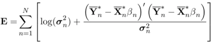
endogenously and compute an entropy measure:

E

=

N

X

n=1

2

6

4

log(

) +

Y

X

Y

X

n

3

7

5

for each case. Higher entropy scores re‡ect poorer performance with relative entropy related

to the familiar likelihood ratio statistic.

Table 2 reports the results of the MC experiments. As expected, less misspeci…cation

is better than more misspeci…cation. Interestingly, knowing the truth (zero misspeci…cation)

is statistically equivalent to estimating the truth (endogenous clustering), with the di¤erences

in the entropy scores likely due to variations in the small sample performances.

Thus, we

conclude that, in cases in which the truth is known, imposing the cluster composition is …rst

best.

However, if the cluster composition is not certain, allowing the data to determine the

clusters reduces the risk of misspeci…cation.

It is important to keep in mind that, in these

experiments, we know with certainty the true number of clusters. If the number of clusters is

unknown, the potential for misspeci…cation increases dramatically.

1.3 Incorporating Prior Beliefs of Cluster Membership

In the previous section, we assumed a ‡at prior over cluster membership.

There

are cases, however, for which prior information could be useful in characterizing the clusters.

For example, similar industrial composition or geographic proximity could lead countries to

respond to the same common factor. In this section, we consider an alternative logistic prior

for the cluster membership indicator,

.

For this multinomial prior, we include additional

1 2_{The entropy measure is calculated for each Gibbs iteration and the mean over all iterations is reported. Each}

blocks consisting of the hyperparameters

and

and the latent vector . As in Hamilton and

Owyang (2009), we can think of the prior hyperparameters as population parameters signifying

the clusters’relationships.

1.3.1 Adding a prior for cluster membership

Suppose there exists a vector,

z

, of variables which may in‡uence whether a series

n

belongs to cluster

i

. We assess the probability that series

n

belongs to cluster

i

as

Pr [

= 1

_j

z

] =

8

>

>

<

>

>

:

exp

z

=

h

1 +

P

exp

z

i

i

= 1

; :::; M

1

1

=

h

1 +

P

exp

z

i

i

=

M

;

(6)

for

n

= 1

; :::; N

and where we have normalized

= 0

for identi…cation. In the multinomial

framework, series

n

cannot be a¢ liated with more than one idiosyncratic cluster. Note also that

the vector,

z

, need not be composed of the same variables for each cluster

i

. The standard

approach to estimating the multinomial logistic is to augment the system in the spirit of Tanner

and Wong (1987) with a latent vector that has the characteristic that the nonnegative element

also re‡ects the cluster to which series

n

belongs. Formally, let

= (

; :::;

)

denote a set

of latent vectors such that

ni

0

if

= 1

<

0

otherwise

:

(7)

Suppose that

has the limiting distribution of the Kolmogorov-Smirnov test statistic:

p

(

) = 8

X

j=1

( 1)

j

exp

2

j

:

(8)

If

KS

and

o

N

(0

;

1)

, then

=

z

0

ni i

+ 2

o

has a logistic distribution with mean

z

and unit scale parameter.

The cluster probabilities can be rewritten in terms of the

new latent variables:

Pr (

>

0) =

exp

z

1 +

P

exp

z

:

The following subsections demonstrate how to draw the hyperparameters governing the

cluster prior probabilities.

1.3.2 Augmenting the Sampler

The sampler outlined in Section can be augmented to account for the logistic prior

described above.

Conditional on the

’s, draws of most of the model parameters remain

unchanged. The change to the logistic prior does alter the acceptance probability in the joint

draw of

and

to the probability de…ned by

(6)

.

The only other modi…cation is in the

form of two additional blocks sampling the three prior parameters: covariate e¤ects,

; the

logistic variances,

; and the vector of latent variables, .

Each of these blocks is drawn by

iterating (jointly) over the

M

1

unnormalized clusters.

1 3

1.3.2.1 Generating

_j

; ; ;

F;

Y

Conditional on

and

,

are the slope coe¢ cients from a standard Normal regression

model for each of the form:

i

=

Z

+

v

;

where

Z

= [

z1

; :::;

z

]

,

v

N

(

0;

)

, and

=

diag

[

; :::;

]

. We assume a normal prior

for the logistic slope parameters,

N

(

d

;

D

)

.

Thus, the covariate e¤ects can be drawn

from the posterior

j

Y;

;

F

N

(

d

;

D

)

, where

d

=

D

+

Z

Z

1

D

d

+

Z

and

D

=

D

+

Z

Z

1

:

1.3.2.2 Generating

and

_j

; ;

F;

Y

If we condition on

, then

would be Normal,

;

N

(

m

;

)

, for the

i

= 1

; :::; M

1

unnormalized clusters.

The mean of the Normal distribution re‡ects this

normalization:

m

=

z

0

ni i

Without that conditioning but given

,

is a truncated logistic with mean

m

.

The

truncation point is at zero, where

determines the direction of the truncation:

0

if

ni

= 1

and

<

0

if

= 0

.

from a Generalized Inverse Gaussian distribution. The candidate,

^

, is accepted or redrawn

based on the algorithm described by Holmes and Held (2006).

1.4 Empirical Application

As an empirical application, we reconsider the model proposed in KOW in which

geography is the sole determinant of cross-country comovements. We include in the hierarchical

prior sets of variables which have been suggested to a¤ect trade between countries. In doing

this, we can assess the sources of business cycle comovements.

1.4.1 Data

Our measure of business cycle activity is the annual constant-price chain-weighted real

GDP growth rate (computed as the di¤erence in the log of real GDP) taken from the 6.3 version

of the Penn World Tables [Heston, Summers, and Aten (2009)].

To maintain comparison, we

choose the same 60 countries located in seven regional blocks from KOW.

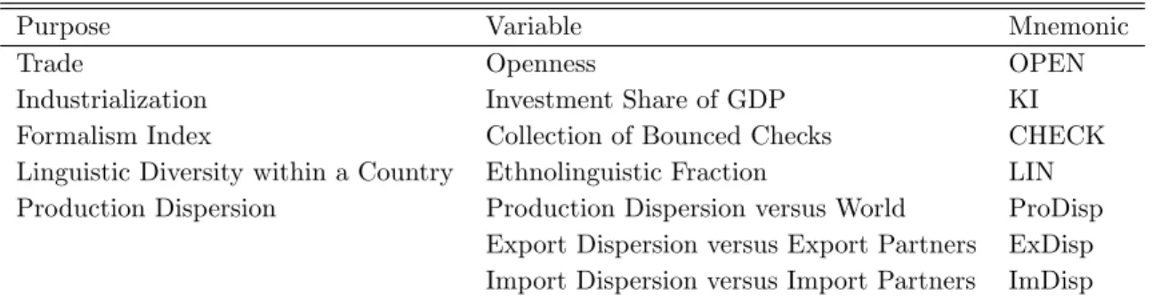
In addition to the real GDP data, the use of the logistic prior requires covariate data,

Z

.

Our covariate dataset includes domestic and international variables as well as indices of

institutional di¤erences.

We will focus on the di¤erences in legal and linguistic institutions.

We have a total of seven covariates that inform the logistic prior: (1) The degree of economic

openness, de…ned as the ratio of imports and exports to GDP; (2) Investment share of real

GDP; (3) An index of con‡ict resolution and sophistication of the legal system as captured

1 4

KOW’s business cycle data include other series in addition to real GDP, allowing them to estimate country

factors. We focus on the comovements across countries by restricting the model to a single business cycle

indicator. Extension to include country factors is left for future research.

1 5

by the manner in which lower courts facilitate landlords’collection of checks (and remedies for

bounced checks); (4) An index of language diversity within each country; (5) An index of

production dispersion relative to the rest of the world; (6) An index of export dispersion from

each country’s exporting partners;

and (7) A similar index of import dispersion from each

country’s importing partners. The covariate data are summarized in Table 3.

Openness measures the size of trade as a fraction of GDP. This variable proxies the

extent of a country’s dependence on foreign economies and exposure to external shocks,

with-out controls for the types of goods traded or the identities of trading partners, allowing us to

determine whether countries cluster based on the (relative) extent of their (direct) exposures

to international shocks.

Investment share of GDP is meant to capture the degree of

indus-trialization; similar levels of industrialization may make countries susceptible to similar shocks

inducing comovements.

The indices in (3) and (4) are included to test the extent to which institutions matter

for clustering.

Our institutional variables are the level of formality of the civil-court system

and the degree of linguistic-diversity. Djankov et al. (2003) construct the lower court system’s

formalism

index in (3) which

"measures substantive and procedural statutory intervention in

judicial cases at lower-level civil trial courts [p.469]"

. We hypothesize that trade ‡ow between

countries with similar con‡ict resolution processes in civil courts could be higher as individuals

may prefer to form relationships in countries with familiar legal set-ups.

The ethnolinguistic index in (4) is taken from La Porta et al. (1999) and measures the

degree of language diversity, the probability that two randomly selected individuals in a given

country speak di¤erent languages, are not speaking the o¢ cial language, or are not speaking

the most widely used language.

how the composition of a country’s production and trade di¤er from the rest of the world and

its trading partners. These indices are akin to variance measures, with the exception that the

export and import dispersions are weighted by sectoral export and import shares. A look at

the trade dispersion indices, (6) and (7), reveals that they capture both the strengths of trading

relations with di¤erent countries and the strength in the diversity of goods traded.

_Baxter

and Kouparitsas …nd that industrialized nations have dispersions similar to the rest of the world

(the average country) for all three indices while developing countries systematically have higher

values of dispersions. On the trade side, this is consistent with the fact that the bulk of trade

of an industrialized nation is with other industrialized nations, while developing nations have

trade relations more evenly spread across developed and developing nations.

By including

these indices, we are allowing for the possibility that countries cluster on the similarities in

their production structures (in terms of types of goods produced) and/or on the compositions

of their trade (both in terms of types of goods traded and the trading partners).

1.4.2 Results

We …rst determine the optimal number of country clusters which, for simplicity, we

compute with a ‡at hierarchical prior on cluster membership.

This allows us to determine

the optimal number of clusters based solely on the business cycle properties of GDP. With

‡at model priors, the Bayes factors are identically the posterior odds. Table 4 presents these

results.

The model with the highest probability is the model with three clusters.

Two and

six clusters have the next highest marginal likelihood; however either alternative require more

than 100 times higher prior likelihood to be preferred.

The model with seven clusters – the

speci…cation which nests the one estimated by KOW – has one of the lowest likelihood of the

1 6

alternatives tested.

We now estimate the model using the logistic prior for the speci…cation with three

regional factors and one global factor.

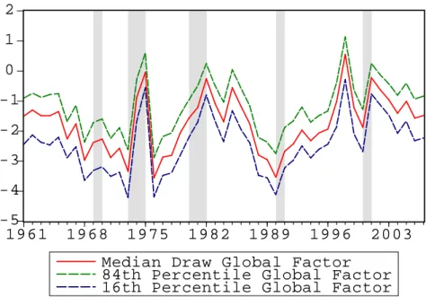
Figure 1 plots the median of the global factor along

with its 16th and 84th percentiles; the shaded areas show the NBER-de…ned recession dates

de…ned as a year in which any quarter was in recession. While the NBER recessions are de…ned

only for the U.S., they serve as reference points. The global factor roughly represents a global

cycle with most countries’ factor loadings being negative.

The global factor spikes around

1975, 1982, 1998, and 2001. With the exception of 1998, these periods are roughly associated

with U.S. NBER recessions.

Figure 2 shows the …rst cluster factor along with its 68 percent probability bands and

the NBER recessions. Figure 3 shows the posterior inclusion probabilities for this cluster. Dark

blue indicates countries which are very likely to be included in this cluster. Yellow indicates

countries which are very likely not associated with the cluster.

Countries in white are not

included in our sample. Note, in particular, that this cluster does appear to demonstrate some

regional/geographic properties. The cluster includes, with high probability, Japan and many

of the countries in Europe. Some European countries –e.g., Iceland and Ireland –belong with

more than 50 percent probability. Brazil, Thailand, and Pakistan also belong with more than

50 percent probability.

Not all of the European countries, however, appear to belong to this

cluster. In particular, the U.K. and Denmark are excluded.

Figure 4 shows the second cluster factor. This factor clearly appears to decline around

NBER recessions. Figure 5 shows why.

The U.S. belongs to this cluster with probability 1;

the cluster also includes Australia, Canada, Hong Kong, India, Malaysia New Zealand, and the

1 7_{In this case, the algorithm chooses nearly empty clusters at some Gibbs iterations, suggesting that seven}

U.K. with very high posterior probability. Also included in this cluster are Denmark and many

of the sub-Saharan African countries including South Africa.

Figure 6 shows the …nal factor and Figure 7 shows the composition of its cluster. Again,

the cluster displays some regional/geographic characteristics with some notable exceptions.

The cluster includes with high probabilities most of the countries in South America, with the

exception of Brazil. Mexico, the Philippines, and a few African countries also belong with high

probability.

As opposed to a purely continental approach such as KOW, our results suggest that a

country like Mexico is much more likely to belong have similar cycles to its common language

South American neighbors than its more geographically proximate neighbor, the U.S. These

results suggest that common culture – either through linguistic or legal similarities – matter

more for cyclical commonality than iceberg costs usually associated with geographic proximity.

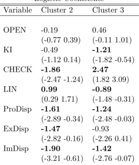
Table 5 shows the posterior means for the logistic covariates along with the 16th and 84th

percentiles of the posterior distributions. The level of industrialization proxied by the country’s

investment share of GDP is important in determining the clusters.

Also, similarities in the

countries’ legal systems and in their linguistic diversity also appear relevant.

This view is

consistent with the notion that trade ‡ows –and, therefore, business cycle comovements –are

more likely across countries with similar institutions.

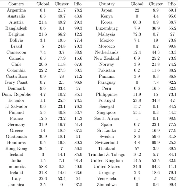
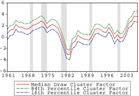
more industrialized countries. Moreover, they conclude that the regional factors explain only

a very small portion of macroeconomic ‡uctuations (about 3.6 percent on average of the 60

countries’ output ‡uctuations).

Our results suggest that there exists a much larger role for

the “regional”factor if region is estimated by the countries’cyclical commonality. In fact, our

cluster factors explain an average of 22.5 percent of the countries’output ‡uctuations.

There are a few reasons this di¤erence may not be surprising. First, KOW’s regional

factors are de…ned as the common component for three series for each country. The inclusion

of the additional two macroeconomic series could potentially contaminate their regional factor’s

ability to explain output ‡uctuations.

Second, imposing rather than estimating the regions

may lead to the same misspeci…cation discussed in the Monte Carlo experiments above. When

countries are included in a region with countries which it does not actually share a common

factor, the factor and the associated loadings may be biased.

1.5 Conclusions

A great deal of research has been done on measuring the comovement of business cycle

variables across countries. Limited by the potential proliferation of the estimated parameters,

these empirical models typically (1) compare business cycles which are estimated

country-by-country; (2) use models of relatively few countries (e.g., bilateral analyses); and/or (3) impose

the structure of the correlations

ex ante

.

One application of the latter, KOW, estimates a

factor model in which the correlation structure across countries is assumed to be determined

by geographic proximity – that is, countries which share a continent also share a common

unobserved factor.

1.6 Tables and Figures

Priors for Estimation - I

Parameter

Prior Distribution

Hyperparameters

n

N

(

b

;

B

)

b

=

0

I

;

B

=

I

8

n

2

n 20

;

0

2 0

= 6 ;

= 0

:

1

8

n

n

U

(

)

or

Logistic

=

8

n

N

(

v0;

V

)

v0

=

0

;

V0

=

1

2

I

8

i

N

(

w0;

W

)

w0

=

0

;

W0

=

1

2

I

8

n

i

N

(

d0;

D0

)

d0

=

0

I7

;

D0

=

2

I7

Table 1: Priors for Estimation - I. Notes: n denotes the series. i indicates the cluster, where

M is the total number of cluster factors. p’s are the maximum number of lags in the error and

factor lag polynomials.

Cluster Misspeci…cation

60%

40%

20%

6

:

7%

5%

3

:

4%

1

:

7%

N one

Endo

Entropy

Table 2: Cluster Misspeci…cation. Notes: The table reports the median for 1000 Monte Carlo

replications with sample size of 50 periods. Unless otherwise speci…ed, each sample contains 60

series, 5 cluster factors, and 1 global factor. The panel compares the results from the endogenous

cluster algorithm to the exogenous cluster algorithm for di¤erent degrees of missepci…cation.

The column headers indicate the percent of the series in the exogenous clusters are misallocated.

’None’speci…es the exogenously clustered model with known clusters. 1 misallocated series out

of 60 equates to 1.66 percent misspeci…cation, etc.

Covariate Data

Purpose Variable Mnemonic

Trade Openness OPEN

Industrialization Investment Share of GDP KI

Formalism Index Collection of Bounced Checks CHECK

Linguistic Diversity within a Country Ethnolinguistic Fraction LIN

Production Dispersion Production Dispersion versus World ProDisp

Export Dispersion versus Export Partners ExDisp

Import Dispersion versus Import Partners ImDisp

Model Choice

ln

f

(

Y

_j

)

ln

(

)

ln

_b

(

_j

Y

)

ln

m

_b

(

Y

)

Odds

f

= 2

-6772

-2173

211

-9157

-58

f

= 3

-6746

-2193

159

-9099

0

f

= 4

-6893

-2206

114

-9214

-115

f

= 5

-6999

-2221

91

-9312

-213

f

= 6

-6879

-2229

12

-9121

-22

f

= 7

-7008

-2236

55

-9301

-202

Table 4: Model Choice. Notes: The table shows the log marginal likelihood for model with

various numbers of clusters estimated with the empirical data. The third column shows the

di¤erence in the log marginal likelihoods between the best model and each other model. The

last column shows how much more likely the best model is compared to each other model.

Logistic Coe¢ cients

Variable

Cluster 2

Cluster 3

OPEN

-0.19

0.46

(-0.77 0.39)

(-0.11 1.01)

KI

-0.49

-1.21

(-1.12 0.14)

(-1.82 -0.54)

CHECK

-1.86

2.47

(-2.47 -1.24)

(1.82 3.09)

LIN

0.99

-0.89

(0.29 1.71)

(-1.48 -0.31)

ProDisp

-1.61

-1.24

(-2.89 -0.34)

(-2.48 -0.03)

ExDisp

-1.47

-0.93

(-2.82 -0.16)

(-2.26 0.41)

ImDisp

-1.90

-1.42

(-3.21 -0.61)

(-2.76 -0.07)

Variance Decompositions - Posterior Means

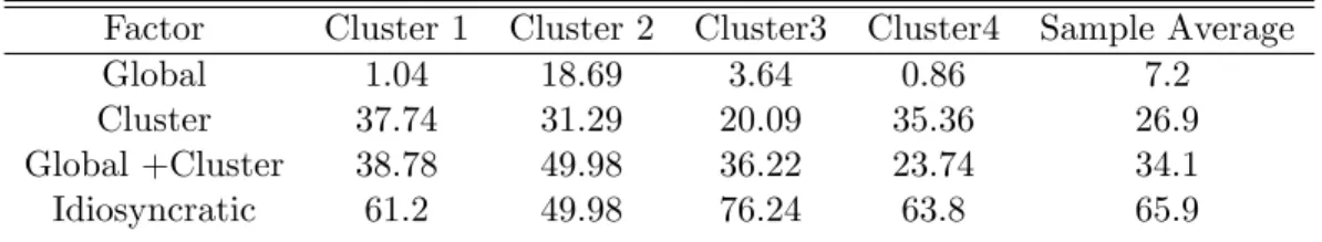
Country Global Cluster Idio. Country Global Cluster Idio.

Argentina 0.1 21.7 78.2 Japan 22 8.9 69.1

Australia 6.5 49.7 43.8 Kenya 0 4.4 95.6

Austria 21.4 49.2 29.3 Korea 60.3 0.9 38.7

Bangladesh 0.6 0.1 99.3 Luxemburg 7.9 36.9 55.2

Belgium 21.6 66.2 12.2 Malaysia 72.3 0.7 27

Bolivia 3.1 19.5 77.4 Mexico 7.1 19 73.8

Brazil 5 24.8 70.3 Morocco 0 0.2 99.8

Cameroon 7.4 3.7 88.9 Netherlands 12.4 44.3 43.3

Canada 6.5 77.9 15.6 New Zealand 0.9 25.2 73.9

Chile 20.6 11.8 67.6 Norway 3.9 21.8 74.2

Colombia 22.2 27.3 50.5 Pakistan 0.2 11.6 88.2

Costa Rica 0.9 28 71.2 Panama 3.9 9.3 86.8

Ivory Coast 0.7 2.5 96.8 Paraguay 0 7.8 92.2

Denmark 9.6 33.4 57 Peru 0.6 16.5 82.9

Dom. Republic 4.7 10.2 85.1 Philippines 11.9 15 73.1

Ecuador 1.1 25.5 73.5 Portugal 23.8 34.3 42

El Salvador 0.6 23.1 76.3 Senegal 15.7 0.1 84.2

Finland 5.5 40.8 53.7 Singapore 55.1 0.3 44.5

France 12.5 73.2 14.3 South Africa 1 0.1 98.9

Germany 31.9 16.7 51.4 Spain 0.7 22.1 77.2

Greece 14 18.5 67.5 Sri Lanka 5.2 16.9 77.9

Guatemala 30.9 18.1 51 Sweden 8.6 59.6 31.8

Honduras 0.5 19.3 80.2 Switzerland 4.8 69.9 25.3

Hong Kong 36.4 7 56.5 Thailand 57 3.9 39.2

Iceland 0 14.1 85.9 Trinidad & Tobago 10.2 5.7 84.1

India 1.5 7.1 91.4 United Kingdom 14.5 52.5 32.9

Indonesia 58.8 0.3 40.9 United States 24.6 64.3 11.1

Ireland 21.8 14.6 63.6 Uruguay 2.3 18.6 79.1

Italy 22.6 53.4 24 Venezuela 0.4 21 78.5

Jamaica 2.5 0 97.5 Zimbabwe 0 0.6 99.4

-5

-4

-3

-2

-1

0

1

2

1961

1968

1975

1982

1989

1996

2003

Median Draw Global Factor

84th Percentile Global Factor

16th Percentile Global Factor

-5

-4

-3

-2

-1

0

1

2

3

1961

1968

1975

1982

1989

1996

2003

Median Draw Cluster Factor

84th Percentile Cluster Factor

16th Percentile Cluster Factor

Figure 2: Cluster 1 Factor. Notes: The red solid line is the median of the posterior distribution

of Cluster 1’s factor. Dashed lines represent the 16th and 84th percentiles. Shaded regions are

annual NBER recessions, where a recession is de…ned as a year in which any quarter was in

recession according to the Business Cycle Dating Committee turning points.

-4

-3

-2

-1

0

1

2

3

4

1961

1968

1975

1982

1989

1996

2003

Median Draw Cluster Factor

84th Percentile Cluster Factor

16th Percentile Cluster Factor

Figure 4: Cluster 2 Factor. Notes: The red solid line is the median of the posterior distribution

of Cluster 2’s factor. Dashed lines represent the 16th and 84th percentiles. Shaded regions are

annual NBER recessions, where a recession is de…ned as a year in which any quarter was in

recession according to the Business Cycle Dating.

-6

-4

-2

0

2

4

6

1961

1968

1975

1982

1989

1996

2003

Median Draw Cluster Factor

84th Percentile Cluster Factor

16th Percentile Cluster Factor

Figure 6: Cluster 3 Factor. Notes: The red solid line is the median of the posterior distribution

of Cluster 3’s factor. Dashed lines represent the 16th and 84th percentiles. Shaded regions are

annual NBER recessions, where a recession is de…ned as a year in which any quarter was in

recession according to the Business Cycle Dating Committee turning points.