ON THE USE OF ENTROPY PRODUCTION TO IMPROVE MATHEMATICAL MODELS AND NUMERICAL METHODS FOR NON-DILUTE FLOW AND TRANSPORT IN POROUS MEDIA
Timothy M. Weigand
A dissertation submitted to the faculty of the University of North Carolina at Chapel Hill in partial fulfillment of the requirements for the degree of Doctor of Philosophy in the Department of
Environmental Sciences and Engineering.
Chapel Hill 2020
ABSTRACT
Timothy M. Weigand: On the Use of Entropy Production to Improve Mathematical Models and Numerical Methods for Non-Dilute Flow and Transport in Porous Media
(Under the direction of Cass T. Miller)
Non-dilute flow and transport in porous media plays an important role in many natural and engineered systems, however a mature understanding is lacking. As environmental conditions change and water resources become scarcer, the need for a more complete understanding of non-dilute flow and transport will be necessary to address future challenges, for example, assessing impacts of climate change on fresh water supplies and examining mitigation strategies. The thermodynamically constrained averaging theory (TCAT) is an approach for developing mathematical models that ties together
ACKNOWLEDGEMENTS
TABLE OF CONTENTS
LIST OF TABLES . . . ix
LIST OF FIGURES . . . x
LIST OF ABBREVIATIONS . . . xiii
LIST OF SYMBOLS . . . xiv
CHAPTER 1: INTRODUCTION . . . 1
1.1 Non-Dilute Flow and Transport . . . 1
1.2 Non-Dilute Flow and Transport Models . . . 2
1.2.1 Length Scales . . . 2
1.2.2 Existing Models . . . 2
1.2.3 Thermodynamically Constrained Averaging Theory . . . 3
1.3 Subscale Modeling . . . 4
1.4 Numerical Methods for Non-Dilute Flow and Transport Problems . . . 5
1.5 Research Objectives . . . 6
CHAPTER 2: MODELING NON-DILUTE TRANSPORT USING THE THERMODY-NAMICALLY CONSTRAINED AVERAGING THEORY . . . 8
2.1 Introduction. . . 8
2.2 Experimental Materials and Methods . . . 11
2.2.1 Materials . . . 12
2.2.2 Measurement Methods . . . 12
2.2.3 Displacement Experiment Methods . . . 13
2.3 Model Formulations . . . 14
2.3.1 Fickian Model . . . 15
2.3.3 Thermodynamically Constrained Averaging Theory Model . . . 17
2.3.4 Additional Relations . . . 20
2.4 Model Solution . . . 21
2.4.1 Model Approximation . . . 21
2.4.2 Parameter Estimation . . . 24
2.4.3 Computational Environment . . . 24
2.5 Results and Discussion . . . 24
2.5.1 Equations of State . . . 24
2.5.2 Displacement Experiments . . . 25
2.5.3 Dilute Flow and Transport . . . 28
2.5.4 Non-Dilute Parameter Estimation Results . . . 29
2.5.5 Forward Simulation Results . . . 33
2.5.6 Components of Mass Flux . . . 35
2.5.7 Model Alternatives . . . 39
2.5.8 Limitations . . . 39
2.6 Summary and Conclusions. . . 40
CHAPTER 3: A PHYSICALLY-BASED ENTROPY PRODUCTION RATE METHOD TO SIMULATE SHARP FRONT TRANSPORT PROBLEMS IN POROUS MEDIA . . . 41
3.1 Introduction. . . 41
3.2 Objectives . . . 42
3.3 Background . . . 43
3.4 TCAT Formulation . . . 46
3.4.1 Non-Dilute Species Transport Model . . . 46
3.4.2 Dilute Species Transport Model . . . 49
3.4.3 Entropy Production Rates . . . 49
3.5 Solution Approach . . . 50
3.5.1 Finite Element Formulation . . . 50
3.5.3 Dilute Model . . . 54
3.5.4 Non-Dilute Model . . . 56
3.5.5 Implementation Details . . . 57
3.6 Results and Discussion . . . 58
3.6.1 Dilute Species Transport . . . 58
3.6.2 Non-Dilute Species Transport . . . 63
3.7 Conclusions. . . 69
CHAPTER 4: MICROSCALE MODELING OF NON-DILUTE FLOW AND TRANSPORT . . . 71
4.1 Introduction. . . 71
4.2 Objectives . . . 72
4.3 Background . . . 72
4.4 Model Formulation, Approximation, and Application . . . 75
4.4.1 Microscale Model . . . 75
4.4.2 Non-dimensional Microscale Model . . . 76
4.4.3 Macroscale Model . . . 77
4.4.4 Model Approximations . . . 79
4.4.5 Microscale Domain Generation . . . 80
4.4.6 Model Implementation . . . 80
4.5 Results and Discussion . . . 83
4.5.1 Dilute Simulations . . . 83
4.5.1.1 Dilute REV-Scale Simulations . . . 83
4.5.1.2 Dilute Sub-REV-Scale Simulations . . . 84
4.5.2 Non-Dilute . . . 85
4.5.2.1 Non-Dilute REV-Scale Simulations . . . 85
4.5.2.2 Non-Dilute Sub-REV Simulations . . . 90
4.5.3 Isolation of Phenomena . . . 94
4.5.3.1 Activity . . . 96
4.5.3.3 Density . . . 97
4.5.4 Macroscale Models . . . 98
4.6 Conclusions. . . 99
CHAPTER 5: CONCLUSIONS . . . 100
5.1 Conclusions. . . 100
5.2 Future Work . . . 101
APPENDIX 1: DETAILED TCAT NON-DILUTE MODEL FORMULATION . . . 103
LIST OF TABLES
2.1 Experimental conditions for displacement experiments showing the difference
in the fluid properties between the displacing and displaced fluids. . . 26
2.2 Fitted Longitudinal Dispersivity. . . 28
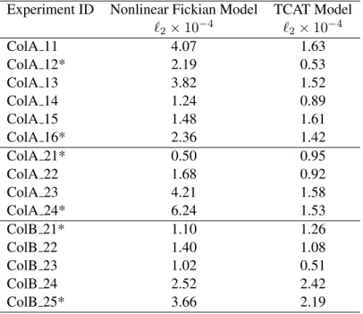
2.3 Forward Simulation Results for Both Models and Columns . . . 34
3.4 Average Convergence Rate for the Dilute Simulations . . . 59
3.5 Average Convergence Rate for the Non-Dilute Simulations . . . 65
4.6 Experimental values and optimized macroscale parameters for the REV-scale dilute simulations. . . 84
LIST OF FIGURES
2.1 Results from fitting the Fickian dispersion coefficient with the dilute flow and transport model for the least and most disperse scenarios. The least disperse experiment had an incoming CaBr2mass fraction of 0.4 and pure water as the
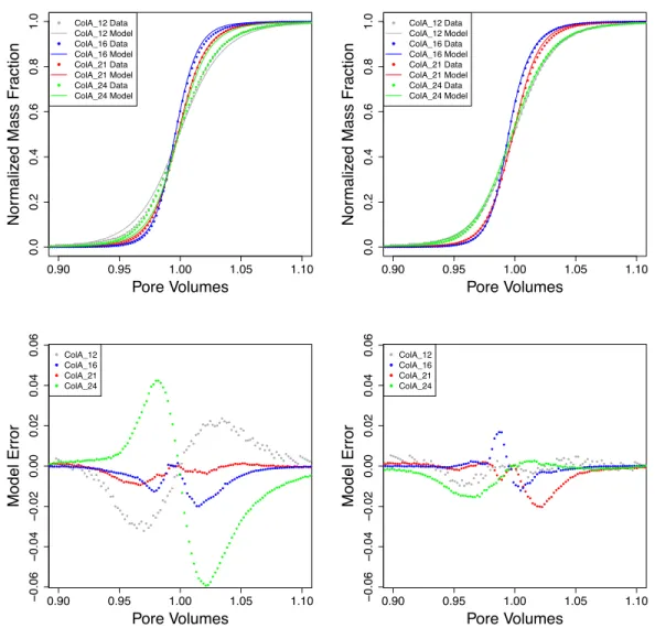
resident fluid. . . 29 2.2 Parameter estimation results and error for the nonlinear Fickian Model (left)
and the TCAT model (right) for Column A. . . 30 2.3 Parameter estimation results and error for the nonlinear Fickian model (left)
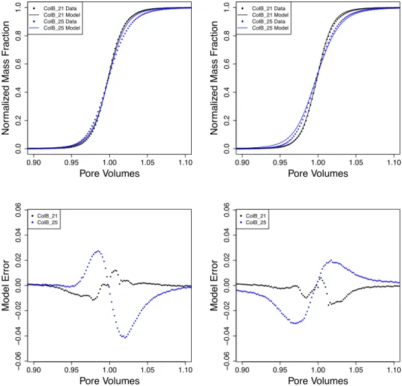
and the TCAT model (right) for Column B. . . 32 2.4 Forward simulations results and model error for the nonlinear Fickian model
(left) and the TCAT model (right) for experiments when pure water was initially
in the column. . . 35 2.5 Forward simulations results and model error for the nonlinear Fickian model
(left) and the TCAT model (right) for experiments when brine was initially in
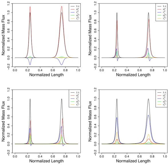
the column. . . 36 2.6 The four flux terms and the sum of the fluxes, for a low (top left), medium
(top right), high (bottom left) concentration displacement, and a displacement
experiment where brine is initially in the column (bottom right). . . 37 2.7 The skewness of the outflow concentration for all simulations for the laboratory
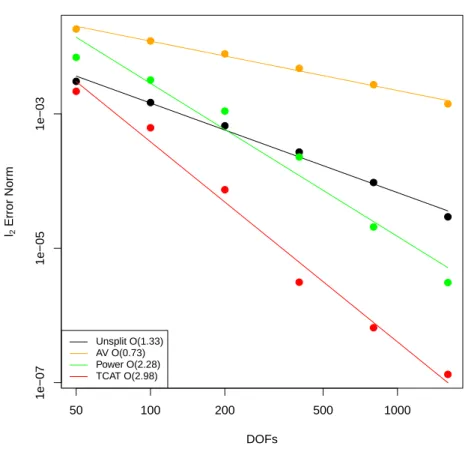
data and the Nonlinear Fickian and TCAT models. . . 38 3.8 Convergence for the largest Pe and the alternating split-operator algorithm for
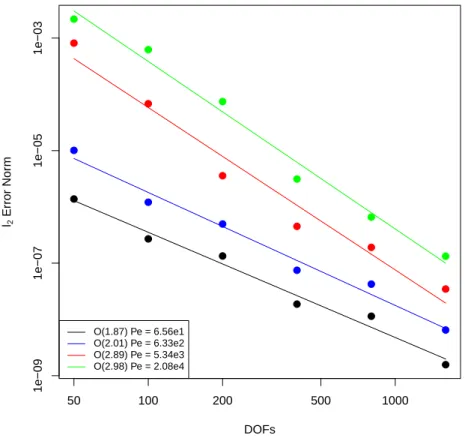
the dilute model. . . 59 3.9 Convergence for the TCAT alternating split operator-approach for each Pe
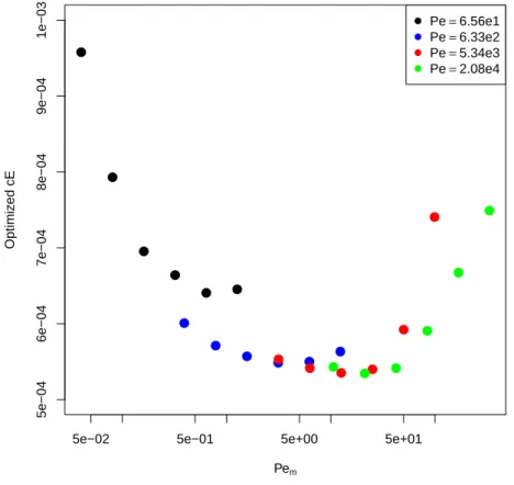
Number for the dilute model. . . 60 3.10 OptimizedcE for the TCAT alternating split-operator approach for the dilute model.. . . 61
3.11 Error for the dilute TCAT approach with the alternating split-operator approach for optimized (filled circles) and averaged (non-filled circles) values of thecE
parameter vs the mesh Pe number. . . 62 3.12 Solution and entropy residual (R) for the dilute model for the largest Pe using
the alternating split-operator approach with 400 DOFs (dashed) and 800 DOFs (solid). . . 63 3.13 Dense grid solutions for the experiments considered for the TCAT non-dilute
flow and transport model. . . 64 3.14 Convergence of the alternating split-operator, TCAT-viscosity approach for the
3.15 OptimizedcE for the alternating split-operator, TCAT-viscosity approach for
the non-dilute model. . . 66 3.16 Difference between`2 error norms for optimized and averagedcE for the
alternating split-operator, TCAT-viscosity approach. . . 67 3.17 Solutions obtained using the alternating split-operator algorithm for both EV
approaches with 400 DOFs. . . 68 3.18 Solution and nodal entropy residual for an incoming mass fraction of 0.2 and
pure water resident fluid for the alternating split-operator approach with 400
DOFs (dashed) and 800 DOFs (solid). . . 70 4.19 Sphere packing results (a) and grain diameter distribution (b) for the REV-scale
domain. The direction of flow for all simulations was upwards and the blue
box represents the domain that was simulated. . . 81 4.20 Sphere packing results (a) and grain diameter distribution (b) for the
sub-REV-scale domain. The blue box represents the domain that was simulated. . . 82 4.21 Results of fitting the dilute macroscale model (lines) to REV-scale cross-section
averaged microscale data (points) for Pe = 0.026 (a), 2.6 (b), and 260 (c). . . 85 4.22 Dilute microscale sub-REV velocity distributions for Re0 = 3.1×10⁻⁵ (a)
and Re0 = 0.31 (b). The means and standard deviations of the velocity are included. The distributions were sampled at a cross-section orthogonal to the
mean direction of flow. . . 86 4.23 Laboratory experiments (a) from (Weigand et al., 2018a) and averaged
REV-scale microREV-scale simulations (b). Both the laboratory experiments and simula-tions use CaBr2as the salt species but the results shown are at different Re and
the column lengths differ. . . 87 4.24 Averaged REV-scale non-dilute breakthrough curves for Re≈10−3. . . 89 4.25 Molecular diffusion sensitivity to density, viscosity, and activity (see Eqn (4.92)). . . 89 4.26 Normalized microscale mass fraction for the dilute (a) andωin = 0.4 and
ωres = 0(b) experiments at Re≈10−3. The direction of flow is upwards. . . 91 4.27 Velocity and mass fraction distributions forωin= 0.1(a) andωin= 0.4(b) at
Re≈10−3. The fields were sampled at a cross-section orthogonal to the mean
direction of flow. . . 92 4.28 Normalized microscale mass fraction for the dilute (a) and ωin = 0.4 (b)
experiments at Re≈10−1. For the non-dilute displacement, higher density
fluids can be seen above lower density fluids where grains of sand touch. . . 93 4.29 Velocity and mass fraction distributions forωin = 0.4ate Re≈ 10−1. The
velocity field was sampled at a cross-section orthogonal to the mean direction
4.30 REV-scale macroscale breakthrough curves for Re≈10−3(a) and the break-through curves where the activity (b), viscosity (c), and density (d) are switched
to their dilute values. . . 95 4.31 Sub-REV-scale breakthrough curve sensitivity forωin= 0.4(a) andωin= 0.5
LIST OF ABBREVIATIONS
AV artificial viscosity
CEI constrained entropy inequality CFL Courant-Friedrichs-Lewy condition CG continuous galerkin approach DAE differential-algebraic equation
DDD de-aired, deionized, and distilled water DOF degree of freedom
EI entropy inequality
EV entropy viscosity
FEM finite element method
IDA implicit differential-algebraic solver LED local extrema diminishing
ODE ordinary differential equation PDE partial differential equation
PISO pressure-implicit with splitting of operators REV representative elementary volume
SAMOL spatially-adaptive method of lines
SIMPLE semi-implicit method for pressure-linked equations SEI simplified entropy inequality
LIST OF SYMBOLS
Roman Symbols
A area
AD dilute advective operator AT non-dilute advective operator cE TCAT viscosity tuning parameter d rate of strain tensor
d artificial viscosity
d50 mean grain diameter
ˆ
D hydrodynamic dispersion
DD dilute dispersive operator DT non-dilute dispersive operator
ˆ
D0 dilute molecular diffusion coefficient
ˆ
DAw variable molecular diffusion coefficient ˆ
DAwu dispersive closure coefficient related to diffusion velocity
ˆ
DAwv dispersive closure coefficient related to momentum transfer
f flux
F entropy flux
FAw total advective and dispersive flux
Fr Froude number
FT flow operator
g acceleration vector due to an external force, such as gravity
G magnitude of gravity vector
h reference datum
h grid spacing
H1 standard Sobolev space
I identity tensor
I ionic strength
Is index set of species
J mass flux
K transport matrix
ˆ
k intrinsic permeability
`2 error norm
m molality
˙
m mass flow rate
Mh computational mesh
mi lumped mass matrix
Mij consistent mass matrix
M W molecular weight
Ndof number of degrees of freedom
Ng gravity number
p fluid pressure
P non-advective mass flux related to pressure gradient
P1 first order Lagrange polynomials
Pe Peclet number
Pem mesh Peclet number
Q volumetric flow rate
R entropy residual
Re Reynolds number
RG ideal gas constant ˆ
RuAw advective closure coefficient related to momentum tranfer
ˆ
RAw
v advective closure coefficients related to deviation velocity ˆ
Rp closure coefficients related to pressure variations
S support of a basis function
t time
t stress tensor
T transpose operator
ws→w
u diffusion velocity
v velocity
V partial mass volume
x mole fraction
X partial mass volume fraction
z position defined as positive upwards Greek Symbols
ˆ
αL longitudinal dispersivity ˆ
β fitting parameter that accounts for non-dilute behavior
ˆ
γ activity
Γ non-advective mass flux related to activity gradient
Γ0 inflow boundary
w porosity
η entropy function
θ temperature
Λ entropy production rate density
µ chemical potential
ˆ
µ dynamic viscosity
ρ mass density
ˆ
τ tortuosity
φ basis function
ψ acceleration potential (e.g., gravitational potential)
ω mass fraction of a species in an entity
Ωz non-advective mass flux related to mass fraction gradient
Ω Domain
Ωw spatial domain of wetting phase
Subscripts and Superscripts
∗ non-dimensional variable
0 dilute value
b parameter relating to non-linear Fickian model
B species qualifier
EV entropy viscosity approximation
D non-advective mass flux due to dispersion
Dm non-advective mass flux due to molecular diffusion
g Galerkin solution
in displacing/incoming fluid
L low order approximation
res resident fluid
T parameter relating to TCAT model
CHAPTER 1: INTRODUCTION
1.1 Non-Dilute Flow and Transport
The flow and transport of fresh and saline water in porous media play an important role in many natural and engineered environments. Seawater intrusion, or the displacement of fresh groundwater by saline water, can result in the contamination of fresh water supplies that are used for human con-sumption or to meet agricultural demand (Barlow and Reichard, 2010; Werner et al., 2013). Toxic and radioactive materials are often injected in subsurface rock salt formations as a disposal method (Kolditz et al., 1998; Oldenburg and Pruess, 1995). Brines, or concentrated saline waters, have also been injected into the subsurface as a strategy to prevent migration of dense non-aqueous phase liquids and other toxic chemicals into drinking water supplies (Hill et al., 2001; Miller et al., 2000; Wright et al., 2009).
Recent studies have shown that additional research is required for these applications due to chang-ing environmental conditions and flawed assumptions. For seawater intrusion, climate change and sea level rise will further compound and reduce valuable fresh groundwater reserves (Ketabchi et al., 2016). Rock salts have been shown to not be impermeable to fluid flow, as previously believed, which raises significant concerns for toxic and radioactive waste disposal and the migration of chemicals (Ghanbarzadeh et al., 2015). To address these problems, a mechansitic understanding of the flow and transport of fresh and saline water in porous media is needed.
flow and transport. This term is more general as it includes any chemical species that can affect fluid properties and not just salt.
Non-dilute flow and transport can be viewed as an extension of dilute flow and transport. For a dilute system, the flow and and transport components can be examined independently as the chem-ical species of concern does not impact the flow. The dilute species will move with the fluid while spreading from higher concentrations to lower concentrations due to molecular diffusion. For non-dilute flow and transport, the flow and transport components cannot be isolated because the species of interest affects the fluid properties and the flow field. The movement of the fluid in porous media is al-ready complex when fluid properties are constant due to the tortuous path caused by pore morphology (Bijeljic et al., 2011). When the fluid properties become functions of the species concentration, fluid flow behavior becomes significantly more complicated and additional physical phenomena need to be considered such as gravity stabilization (Fernandez et al., 2002).
1.2 Non-Dilute Flow and Transport Models
1.2.1 Length Scales
The length scale of a model is one of its defining features and in this work we are concerned with the microscale and the macroscale. At the microscale, the smallest of the two scales considered in this work, the exact pore morphology and topology are known as well as the exact boundaries of each phase present in the system (Gray and Miller, 2014). For most practical porous media applications, exact microscale information is unknown. At the macroscale, the phase boundaries are no longer known and a macroscale point is represented by the average microscale conditions among all entities. The averaging region used to determine macroscale variables needs to be sufficiently large such that the average is well-defined and insensitive to small changes in the size of the region. This is known as a representative elementary volume (REV) (Bear, 2012).
1.2.2 Existing Models
Empirical relations are then posed to have a closed system. As an example, many researchers have used the macroscale dilute flow and transport model to simulate non-dilute behavior by forcing the dispersivity parameter to agree with laboratory data (Boufadel et al., 1999; Frolkovic and Schepper, 2000; Ibaraki, 1998). Dispersivity is a measure of how a chemical species spreads due to variations of the microscale velocities but is only a property of the porous medium and not a function of the fluid properties. Rather than deriving a model from a mechanistic understanding of non-dilute behavior, macroscale parameters are forced to describe the empirical evidence thus severely limiting the applica-bility and predictive capabilities of the model (Jiao and H¨otzl, 2004; Konz et al., 2009; Landman et al., 2007a,b; Starr and Parlange, 1976; Watson et al., 2002c).
More formal attempts at developing macroscale models for non-dilute flow and transport in porous media have been unable to provide a mechanistic description of non-dilute behavior and are not de-veloped with a sound fundamental basis (Demidov, 2006; Hassanizadeh and Leijnse, 1995; Landman et al., 2007b). The most popular approach is by Hassanizadeh and Leijnse (1995) that combined aver-aged microscale conservation laws but used macroscale thermodynamics. While models should obey all conservation and thermodynamic laws, the thermodynamic equations should use microscale ther-modynamic equations to have consistency across all spatial scales (Gray et al., 2013). To account for the complex non-dilute microscale behavior, a fitting parameter was introduced that is not explicitly related to any physical phenomena. While the model was able to adequately simulate non-dilute labo-ratory experiments, the usefulness and applicability of the model is reduced as the dependencies and physical phenomena that the fitting parameter represent are unknown (Watson et al., 2002c). There is a need for a macroscale model of non-dilute flow and transport in porous media that begins with a mechanistic understanding of microscale behavior, is developed on a sound fundamental basis and includes, if necessary, parameters that are applicable to a wide range of chemical species and porous media systems.
1.2.3 Thermodynamically Constrained Averaging Theory
to the desired scale. As is often the case, the number of equations is less than the number of unknowns and additional relations are required to obtain a closed model. With TCAT, an entropy inequality is formed to guide the development of the closure relations such that the posited relations must obey the second law of thermodynamics. Evolution equations can be derived from the averaging theorems to ac-count for larger scale geometric quantities that also need closure. The combination of the conservation equations, state equations, entropy-based closure relations, and evolution equations compose a closed, parameterized model.
The TCAT approach ensures that all physical and thermodynamic laws are obeyed. The models are formulated for the most complex scenario and then assumptions are made. This ensures that all assumptions are explicit and that the resulting models reduce to their simpler versions. For example, as the concentration of a species approaches the dilute limit, the non-dilute model should be able to accurately model dilute behavior. As model formulation begins at the microscale, all larger scale equations and variables are written in terms of microscale averages and therefore all variables are well-defined. The sum of these features is unique to TCAT.
Gray and Miller (2009) developed a closed macroscale model for non-dilute flow and transport using TCAT. This model includes all of the features described above and includes physics ignored by other models including dissipative terms related to gradients in activity and pressure. A simulator for this model has not been implemented. Additionally, the relations posited to close the model have not been evaluated and only relate terms through closure coefficients. Parameterization of the closure coefficients is still needed and should be based on a mechanistic understanding of non-dilute behavior.
1.3 Subscale Modeling
Subscale modeling also allows for simulations where specific behavior can be isolated. For exam-ple, if we wanted to examine the effects that density has on non-dilute flow and transport but ignore other aspects such as activity and viscosity, we could simply force the activity and viscosity to be con-stant in the simulations. This is difficult in a laboratory setting as we are constrained to the combined properties of the species selected for the experiments.
Microscale non-dilute flow and transport simulations have been limited to the membrane literature where no porous media is present (Gruber et al., 2011, 2016). Dilute flow and transport in porous media has been studied extensively (Aramideh et al., 2018; Bijeljic et al., 2011, 2004, 2013; Icardi et al., 2014). Using subscale modeling as a tool to improve TCAT models has seen success for two-fluid-phase flow in porous media where closure coefficients have been parameterized, improved state equations have been developed, and enhanced understanding of microscale and macroscale physics has been provided (Bruning and Miller, 2019; Dye et al., 2016; McClure et al., 2017).
1.4 Numerical Methods for Non-Dilute Flow and Transport Problems
Obtaining an accurate solution to the existing macroscale models for non-dilute flow and trans-port is nontrivial (Landman et al., 2007a). The class of problems that include non-dilute flow and transport are known as sharp front problems and the defining feature is an advective term that is large as compared to the dispersive term, if present at all (Farthing and Miller, 2000; Smith et al., 1991; Widdowson et al., 1988). The characteristic of sharp front problems is a near instantaneous transition of the solution variable in space. Low-order numerical methods for sharp front problems will pro-duce a solution free of non-physical oscillations but to obtain an accurate solution, a large number of degrees of freedom are needed to adequately resolve the front (LeVeque, 2002). A large number of degrees of freedom increases the computational cost and for many problems this may not be an op-tion due to computaop-tional constraints and higher order numerical methods are needed. According to Godunov’s theorem, only nonlinear higher-order methods and linear first-order methods can provide non-oscillatory solutions (Godunov, 1959).
2007b; LeVeque, 2002; Miller et al., 2013; Watson et al., 2002c). Many of the nonlinear higher-order methods are not ideal for irregularly shaped domains, which commonly occur in non-dilute flow and transport applications (Miller et al., 2016). Methods where an irregularly shaped domain can easily be incorporated, such as finite element methods (FEM), are not as mature for sharp front problems (Guermond and Popov, 2017; Kuzmin, 2006).
One class of FEM approaches is based on introducing artificial viscosity (or diffusion) into the solution to remove non-physical oscillations (Harten et al., 1976, 1997; Lax, 1971; LeVeque, 1992; Osher and Chakravarthy, 1984; Smoller, 1994). The difficulty with this method is determining the optimal amount of artificial viscosity to introduce; if too little artificial viscosity is included, the so-lution will oscillate, if too much artificial viscosity is added, the soso-lution will be smeared. The op-timal amount of viscosity to add is not knowna priori. One approach for determining the amount of artificial viscosity to include is the entropy viscosity method (EV) that scales the amount of artifi-cial viscosity based on a measure of the mathematical entropy, which is not inherently related to the thermodynamic entropy (Guermond and Nazarov, 2014; Guermond et al., 2010, 2017, 2014, 2011; Guermond and Popov, 2014, 2017). There is no rigorous definition of the optimal entropy function and the choice is problem dependent.
As discussed, an entropy production rate is derived when developing a TCAT model to guide model closure. Pairing the TCAT entropy production rate with the EV method, where a measure of entropy is needed, may produce an efficient solution scheme. This could potentially improve the nu-merical methods used for solving non-dilute flow and transport problems by using the known physics to improve the numerics. This method can easily incorporate irregular boundaries and potentially reduce the high computational cost associated with solving non-dilute flow and transport models.
1.5 Research Objectives
• to develop and solve a parameterized macroscale model to describe non-dilute flow and trans-port in porous media using the thermodynamically constrained averaging theory (Chapter 2); • to improve the numerical methods used to solve the newly developed macroscale model for non-dilute flow and transport in porous media by using the physics to improve the numerical methods (Chapter 3); and
CHAPTER 2: MODELING NON-DILUTE SPECIES TRANSPORT USING THE THERMODY-NAMICALLY CONSTRAINED AVERAGING THEORY
2.1 Introduction
The use of models to describe the flow and transport of non-dilute systems and fresh water is commonplace. Applications include seawater intrusion in coastal aquifers, dense non-aqueous phase liquid remediation and management, and underground injection of hazardous materials (Hill et al., 2001; Kolditz et al., 1998; Miller et al., 2000; Werner et al., 2013; Wright et al., 2009). While existing uses for non-dilute flow and transport models will remain, newer applications are emerging, such as assessing the impacts that climate change and sea level rise will have on fresh water reserves and exploring approaches to mitigate climate change (Ketabchi et al., 2016).
The classical approach for modeling mass transport in porous media for a dilute species involves the use of conservation of mass equations for the fluid and species of interest, Darcy’s law as an approximate conservation of momentum of the fluid, and Fick’s law to represent deviations from the mean flow for the species (Bear, 1979). The form of the dispersion tensor used with Fick’s law consists of a term related to molecular diffusion and a term that is a function of the Darcy velocity weighted by a longitudinal and transverse dispersivity. The dispersivity coefficients are solely func-tions of the porous medium and not a function of the fluid properties. For non-dilute systems, the density and viscosity are functions of the fluid composition, which affects species transport. Therefore, it is understood that the standard Fickian dilute model cannot be applied to non-dilute systems, even for restrictive laboratory cases of a homogeneous isotropic porous media in a system well above the representative elementary volume (REV) scale which is needed for Fickian transport to be a reason-able approximation of reality.
the fluid phase in these systems, Fick’s law has been shown to be inadequate for describing deviations from mean transport for a non-dilute species (Konz et al., 2009; Starr and Parlange, 1976; Watson et al., 2002b; Wright et al., 2009). Dispersion in non-dilute systems has been found to depend on the density gradients, viscosity gradients, and mean flow rate, in addition to properties of the porous media (Broeke and Krishna, 1995; Jiao and H¨otzl, 2004; Konz et al., 2009; Landman et al., 2007a,b; Noordman and Wesselingh, 2002; Starr and Parlange, 1976; Watson et al., 2002c). Due to gravity stabilization, the dispersion is reduced for larger density gradient displacements compared to the dilute transport case, and the density gradient has been shown to be the dominant factor in comparison to the viscosity gradient for systems evaluated to date (Landman et al., 2007a). The effects of chemical activity on non-dilute flow and transport have not been reported in the literature.
While some have applied the standard Fickian dilute model to non-dilute systems despite the inherent issues and shortcomings, others have attempted to develop new models to describe non-dilute species transport (Gray and Miller, 2009, 2014; Hassanizadeh, 1990, 1996; Hassanizadeh and Leijnse, 1995; Landman et al., 2007b). A variety of physical mechanisms can affect the observed behavior of non-dilute systems. Therefore, any new model requires significant validation by comparison to experimental data. Ideally, a model should functionally represent the observed data when parameter estimation is performed and successfully predict species transport in systems for which all parameters have been estimated independently. The wider the variety of conditions a model is exposed to, the more confidence one can have in the usefulness of the model. With these guiding principles in mind, non-dilute species transport models have been developed and evaluated with respect to the operative mechanisms.
experiments used NaCl as the non-dilute species. Multiple flow rates and coarse and medium grain sands were examined as well as different flow regimes including constant head and constant flow rate experiments. The optimized parameter in the nonlinear expansion has been found to be sensitive to the difference between the displacing and displaced fluid densities and has been shown to be a function of the velocity of the fluid, where the log of the parameter varies linearly with the log of the Darcy velocity (Landman et al., 2007b; Watson et al., 2002c).
The model of Demidov (2006) was formulated from the microscale, where the boundaries of all phases are resolved in space and in time, and homogenization was applied to derive a macroscale model. This approach requires knowledge of the characteristic pore morphology and topology and a parameterization of the flow field at the microscale. The model neglects viscosity and activity impacts at both scales. This model has only been applied to one set of numerically generated data (Landman et al., 2007b). Landman et al. (2007b) used the characteristic pore size parameter that appears in the model as a fitting parameter to allow for comparison to the numerically generated data, and an empiri-cal relationship was used to represent the microsempiri-cale flow fluid. An accurate fit for two types of porous media and various flow rates was obtained, however the fitting parameter depended upon system condi-tions.
The homogenization model of Egorov (Landman et al., 2007b) was formulated at the mesoscale, which is a scale above the macroscale used to account for heterogeneity at the macroscale. This model assumes that the dilute flow and transport model is an accurate model at the macroscale for non-dilute systems, which has been shown to be false (Anderson, 1997; Brigham et al., 1961; Hassanizadeh and Leijnse, 1995; Slobod, 1964; Welty and Gelhar, 1991). The macroscale permeability distribution field must be known and homogenization was used to derive a mesoscale model. This model neglects viscosity and activity effects at both scales. As with the homogenization model of Demidov (2006), this model has only been applied to a numerically generated set of data (Landman et al., 2007b) and success of the model was limited.
and an entropy inequality is formulated, through the use of Lagrange multipliers, to provide permissi-bility conditions for closure relations. An entity-based momentum equation, as well as a species-based momentum equation, model was derived (Gray and Miller, 2009). The TCAT model includes disper-sion associated with activity and pressure gradients. This model has not yet been solved or compared to experimental data.
Currently, a mature level of understanding for modeling non-dilute transport has not yet been achieved. Only limited experimental data is available and all models posed to date have some com-bination of limited evaluation and validation or certain limitations in describing non-dilute systems mechanistically. Opportunities exist to advance understanding of non-dilute transport using both exper-imental methods that investigate a broader range of physical conditions than have been considered and alternative approaches for mechanistic modeling of these challenging systems.
The overall goal of this work is to improve the understanding of the behavior of non-dilute species transport in porous medium systems. The specific objectives of this work are: (1) to observe sys-tems with a wide range of variability in fluid density, viscosity, and chemical activity of the reference species; (2) to advance a multiscale model formulation approach for describing such systems; (3) to develop efficient numerical approximation methods for the formulated model; (4) to compare exper-imental observations with the formulated model description in both an explanatory and predictive sense; and (5) to assess the importance of previously neglected phenomena, including species transport due to variations in chemical activity.
2.2 Experimental Materials and Methods
2.2.1 Materials
The materials used for this work included a uniform sand for the porous medium, water as a sol-vent, a radioactive tracer, and a non-dilute solute. A 12/20 Accusand was used for the porous medium, which is a uniform quartz sand with a reported mean particle diameter of 1.105 mm (σ = 0.014 mm), uniformity coefficient of 1.231 (σ= 0.043), and a saturated hydraulic conductivity of 30.19 cm/min (σ=1.00 cm/min) (Schroth et al., 1996). De-aired, deionized, and distilled (DDD) water was used for all experiments and dilutions. Tritium was used as a conservative tracer, and calcium bromide (CaBr2) was the non-dilute solute (Dead Sea Bromine Group).
2.2.2 Measurement Methods
The measurements involved in this work included fluid density, fluid viscosity, and the concentra-tion of the radioactive tracer. The methods used to make these measurements are described in turn.
Density was measured using a density meter (Anton Paar DMA 48), where measurements are typically±0.0001 g/mL. The instrument was calibrated using air (0.0012 g/ml at 25◦C) and DDD water (0.9970 g/ml at 25◦C). The density of the saturated brine was monitored through the course of this work and determined to be 1.7039 g/ml.
For determining the density of the solution as a function of the CaBr2mass fraction, a series of solutions were made to characterize density across the mass fractions of interest. Specifically, 30 solutions were analyzed, including pure water. Solutions of brine and water were made by combining volumetric ratios of saturated brine to DDD water starting at 3.33% brine (i.e., 1 part brine to 14 parts water), increasing the ratio of brine of 3.33% (i.e., 2:13, 3:12, 4:11, etc.), and ending with 100% brine (15:0). To ensure the solutions were mixed properly, the mass of each component was also measured and compared with the expected mass, given the known density of both water and brine. Solutions were allowed to equilibrate overnight prior to measuring. The glass tube in the density meter was rinsed several times with water and ethanol, dried with air, and equilibrated back to the known density of air between each measurement.
Viscosity measurements were used to develop an equation of state between viscosity and CaBr2 mass fraction at 25◦C. Viscosity was measured using a falling ball viscometer (Haake Model B). To verify the measurements, results from the viscometer were compared to standards that spanned the range of the unknowns. The measured viscosity for water was compared to a value from the literature (0.890 mPa·s at 25◦C). The error in the measurement was less than 5%. Similarly, the viscosity was measured for a commercial viscosity standard much higher than that of water (Cannon Instrument Company, General Purpose Viscosity Standard N10, 15.79 mPa·s 25◦C). The error in the measurement was 11%.
A series of solutions were made to characterize viscosity across the CaBr2mass fractions of in-terest. Specifically, 10 solutions were made by combining volumetric ratios of brine to DDD water starting at 10% brine (i.e., 1 part brine to 9 parts water), increasing in 10% increments, and ending with 100% brine. Solutions were allowed to equilibrate overnight prior to measuring. Viscosity mea-surements were made by first adding each solution to the falling ball apparatus. Next, one of the cali-brated balls was dropped through the fluid and the amount of time to travel the length of the apparatus was measured and used to calculate an estimate of the viscosity. A minimum of three measurements were made for each solution. An average of these measurements was used when fitting the data for the equation of state.
To measure the concentration of the radioactive tracer, samples were collected in plastic scin-tillation vials and samples were mixed with Fisher 30% scinscin-tillation cocktail. A Packard 1900TR scintillation counter measured the disintegrations per minute (DPM) for two minutes for the different samples and the results were averaged. These results were then converted to have units of mCi.
2.2.3 Displacement Experiment Methods
A set of stable brine displacement experiments were performed in a column packed with homo-geneous porous media. A cylindrical glass column, 90 cm in length and 2.5 cm in diameter was used. Fluids were pumped through the column using syringe pumps (Harvard Apparatus) equipped with glass, air-tight syringes (Hamilton Model 1100). The Darcy velocity for all experiments was 5 m/day.
of the columns changed and potentially the pore morphology and topology. The porosity for both columns was 0.33, which was determined by weighing the mass of sand added to the column and using the density of the sand (2.65 g/cm3). To calculate the tortuosity (τˆ) for each column, the relation for a random homogeneous isotropic sphere packing was used, which is dependent on the porosity, and was calculated to be 1.33 for both columns (Shen and Chen, 2007).
For the tracer displacement experiments, 2-mL aliquots from the effluent were collected in 10-mL plastic scintillation vials. The experiment continued until at least 1.75 pore volumes had passed through column. The results from the end of the column were normalized by dividing by the radioac-tivity of the incoming fluid.
For the brine displacement experiments, the resident fluid was displaced with a fluid of greater density, such that all displacements were always density stable (i.e.,ρwd > ρwr, whereρwis the density of the fluid, and the subscriptsdandrrefer to the displacing fluid density and resident fluid density, respectively). Two types of experiments were conducted: (1) a series where the resident fluid in the column was pure water and and the concentration of the CaBr2in the displacing fluid was varied; and (2) a series where both the resident and displacing fluid CaBr2 concentrations were varied to result in a constant density difference between the two fluids. This second sequence of experiments had variations in viscosity and chemical activity for each pair of resident and displacing mass fractions to provide a means to examine the importance of changes in these variables. Both types of experiments were conducted in Column A and the second type of experiment was repeated in Column B as the column needed to be repacked midway through the replicates for the second type of experiment.
2.3 Model Formulations
The nomenclature for all variables follows the TCAT convention (Gray and Miller, 2014). A superscript on a variable refers to an intrinsic average of a microscale variable to produce a macroscale variable. A single overbar on the superscript means that the term is a density weighted average of a microscale variable, and a double overbar is a unique average, which is defined. Terms with carats are coefficients that may be determined from experimental data using parameter estimation. Three models are considered: the standard Fickian model, a nonlinear Fickian model, and a TCAT model for non-dilute systems, which are summarized in turn in the sections that follow.
2.3.1 Fickian Model
The classical single-fluid-phase flow and Fickian dilute species transport model for a homoge-neous, isotropic porous media has been used to describe non-dilute flow and transport by allowing the density and viscosity of the fluid phase to vary as functions of the species concentration (e.g. Steefel et al., 2015; Voss, 1984; Wright et al., 2009). This model is composed of a conservation of mass equa-tion for the water phase
∂wρw
∂t =−
∂ ∂z
wρwvw , (2.1)
and a conservation of mass equation for the solute species
∂wρwωAw
∂t =−
∂ ∂z
wρwωAwvw− ∂
∂z
wρwωAwuAw , (2.2)
wherezis positive upwards,w is the porosity,ρwis the density of the water phase,vwis the velocity of the water phase,ωAwis the mass fraction of solute speciesA, anduAwis the deviation velocity
from the mean for speciesA. Darcy’s law is used to solve for the velocity of the fluid phase
wvw =−kˆ
ˆ µ
∂pw
∂z +ρ
wgw
, (2.3)
A Fickian approximation for the mass flux resulting from the deviation velocity can be written as (Bear, 1979)
JAw=wρwωAwuAw=−wρwDˆ∂ω Aw
∂z , (2.4)
whereJAwis defined as the mass flux of speciesAandDˆ is the hydrodynamic dispersion for porous
media systems. The hydrodynamic dispersion consists of a term related to molecular diffusion and a term that approximates variations in the microscale velocity. The most commonly used form in one dimension is
ˆ
D= DˆAw ˆ
τ + ˆαLv
w , (2.5)
whereτˆis the tortuosity of the porous medium, which is defined as the actual distance traveled by a species over a unit length of the medium and is greater than or equal to one,DˆAwis the molecular
diffusion coefficient, andαˆLis the longitudinal dispersivity (Bear, 1979).
2.3.2 Nonlinear Fickian Model
The nonlinear Fickian model approximates the dependency of the dispersion on fluid properties. A series expansion of Fickian model yields
1 + ˆβ
J
Aw
JAw=−wρwDˆ∂ω Aw
∂z , (2.6)
whereβˆis a parameter andDˆ is defined in Eqn (4.103). The nonlinear Fickian model was derived us-ing rational thermodynamics (Hassanizadeh, 1986; Hassanizadeh and Leijnse, 1995), and it is assumed that the chemical potential is solely a function of the mass fraction of the species.
An alternative nonlinear Fickian model can also be written in the following form
JAw =−wρw ˆ
DAw
ˆ
τ + ˆα
B Lvw
!
∂ωAw
∂z , (2.7)
where
ˆ
αBL = 2ˆαL
1 + q
1−4 ˆβwρwαˆ Lvw ∂ω
Aw ∂z
Eqns (2.7) and (2.8) result from assuming that only the mechanical dispersion component of Eqn (2.6) is nonlinear in the dispersive flux and that the molecular diffusion component does not depend upon
JAw, althoughDˆm may depend upon other solution variables.
2.3.3 Thermodynamically Constrained Averaging Theory Model
TCAT is a method for formulating models that provides a firm connection between the microscale, or pore scale, and the macroscale for conservation equations as well as thermodynamics (Gray and Miller, 2005, 2014; Miller and Gray, 2005). A formal averaging approach is used to upscale the mi-croscale conservation and thermodynamic equations to the scale of interest. To solve the closure prob-lem, the conservation equations and thermodynamic relations are combined in an entropy inequality. Explicit, formally-stated approximations are used to simplify the entropy inequality to a strict flux-force form. Closure relations are then posited, constrained by a requirement of consistency with the simplified entropy inequality (SEI), and a closed model results. Parameters in the closure relations can be determined with macroscale data using a parameter estimation approach such as nonlinear regres-sion. Alternatively, due to the connection between all spatial scales, subscale or microscale modeling can be performed to determine the parameters in the closure relations (Gray et al., 2015; Miller et al., 2018b).
TCAT differentiates between primary restrictions, SEI approximations, and secondary restrictions (Gray and Miller, 2014). Primary restrictions specify the thermodynamic theory to be used, the system and scale to be considered, and the physical phenomena to be considered. For this problem, classical irreversible thermodynamics is used to describe both equilibrium and near-equilibrium states. The sys-tem of interest consists of a wetting phase, a relatively immobile solid phase, and an interface between the wetting and solid phase. The properties of the wetting phase are dependent on species composition. The scale of the system of interest is the macroscale and system length scales are well separated. The macroscale is defined at a scale that is consistent with the size of the REV (Gray and Miller, 2009). Additionally, the physical phenomena to be considered are the transport of mass, momentum, and energy for each phase and the interface.
Exam-ples of the approximations made for this system include breaking of average quantities and elimination of terms that are expected to be small Gray and Miller (2009). Secondary restrictions are based on the specific system of interest. In this work, the following assumptions are made: the system is isothermal, the interface between the wetting phase and the solid can be neglected, the wetting phase consists of a speciesAfully dissolved in a solventB, no reactions occur, no diffusion of the species into the solid phase, and the porous media is isotropic.
Miller and Gray (2008) and Gray and Miller (2009) have derived two different TCAT models for non-dilute species transport. One form uses a phase-based conservation of momentum equation, while the other uses a species-based conservation of momentum equation. Both of these models have features that are lacking in other attempts to describe non-dilute flow and species transport including gradients related to the pressure and activity that appear in the species conservation of mass equation. As with all TCAT models, the macroscale variables in these models are expressed explicitly in terms of specific averages of microscale quantities making a firm connection between the pore scale and the macroscale.
The phase-based momentum equation TCAT model for non-dilute species transport from Gray and Miller (2009) was extended in this work to include a cross-coupled closure. This formulation is detailed in the appendix, and the final model formulation is summarized as follows.
The simplified conservation of momentum equation for the fluid is
ˆ
RAwv vw=−w∂p w
∂z −
wρwgw−R Gθw
M WW3 M WA2M WB2
ˆ DvAw∂ω
Aw
∂z
−RGθw xAw
ˆ γAw
!
M WW
M WAM WB
ˆ DAwv ∂γˆ
Aw
∂z
−ωAw
ρwVAw−1
M WW2
M WAM WB
ˆ DvAw∂p
w
∂z , (2.9)
where speciesAis defined as the salt and speciesBis the water,RˆAwv andDˆvAware closure coeffi-cients that need to be parameterized,RGis the universal gas constant,θw is the temperature,M WA
andM WBare the molecular weights of speciesAandB,M WW is the molecular weight of the fluid
The conservation of mass equation for speciesAis
∂wρwωAw
∂t +
∂ ∂z
h
wρwωAw−RˆAwu vwi
− ∂
∂z
w
M WW2
M WAM WB
ρwVAw−1ωAwDˆAwu ∂p w ∂z − ∂ ∂z
wρwRGθw
M WW3
M W2
AM WB2
ˆ DAwu ∂ω
Aw ∂z − ∂ ∂z "
wρwRGθw ωAw
ˆ γAw
!
M WW2 M WA2M WB
ˆ DuAw∂ˆγ
Aw
∂z #
= 0, (2.10)
whereRˆuAwandDˆAwu are non-negative closure coefficients. The conservation of mass equation for the water phase is given in Eqn (2.1).
Preliminary work demonstrated that the cross-coupled terms are not significant for this system, therefore we setDˆvAwandRˆAwu to zero. We defineRˆAwv as
ˆ
RAwv = w2µˆ
ˆ
k (2.11)
so that Eqn (2.9) becomes Darcy’s law, which has been shown to be valid for non-dilute systems (Wat-son et al., 2002b).
The remaining issue deals with the parameterization ofDˆAwu . In addition to satisfying the entropy inequality constraint, the posited model should also reduce to the standard Fickian model for dilute systems in the limit of a small mass fraction for the solute species, and to an established form for non-dilute diffusion in the absence of advective transport. We posit a form that meets these criteria, which resulted from the examination of many potential forms.
For the remaining parameter in the conservation of mass equation for the species, we pose the following form
ˆ
DAwu = M W
2
AM WB2
M W3
WRGθw !
ˆ
DAw
ˆ
τ + ˆα
T Lvw
!
, (2.12)
where
ˆ
αTL= 2ˆαL
1 + r
1−βˆ1Twρwαˆ Lvw ∂ω
Aw
∂z −βˆ2Twρw ω
Aw
ˆ
γAw M WB
M WWαˆLvw ∂
ˆ
γAw ∂z
From the SEI,DˆAwu must be greater than or equal to zero. For our upward stable displacement experiments, the spatial gradient of the mass fraction is always negative, however, the spatial gradient of the activity, at low mass fractions, is positive. To ensure the SEI is obeyed, we restrict the two parameters
ˆ
β1T andβˆ2T
to be greater than or equal to zero and we neglect the activity portion ofαˆTL
when the spatial gradient of the activity is positive, which occurs over a relatively small range of small mass fractions of the salt. The two TCAT parameters are fitting parameters that allow the model to vary the amount of dispersion based on chemical composition.
Thus, the conservation of mass equation for a species becomes
∂wρwωAw
∂t +
∂ ∂z
wρwωAwvw
− ∂
∂z "
w
M WAM WB
M WWRGθw
ρwVAw−1ωAw DˆAw ˆ
τ + ˆα
T Lvw
! ∂pw ∂z # − ∂ ∂z "
wρw DˆAw ˆ
τ + ˆα
T Lvw
! ∂ωAw ∂z # − ∂ ∂z "
wρw ω
Aw
ˆ γAw
!
M WB
M WW
ˆ
DAw
ˆ
τ + ˆα
T Lvw
! ∂γˆAw
∂z #
= 0. (2.14)
For ease of notation, the conservation of mass equation for a species may be rewritten in terms of diffusive and dispersive flux terms related to each spatial gradient
∂
wρwωAw
∂t +
∂ ∂z
wρwωAwvw+PzD +PzDm+ ΩDz + ΩDmz + ΓDz + ΓDmz = 0, (2.15)
where theDsuperscript refers to a dispersive flux andDm refers to diffusive flux, andPz, ΩzandΓz
represent the terms associated with the pressure, mass fraction and activity gradient, respectively.
2.3.4 Additional Relations
For the diffusion coefficient, we used the following form
ˆ
DAw= ˆD0
ˆ µ0
ˆ µ
1
ρwVBw
1 +mAw
dln ˆγAw
dmAw
, (2.16)
whereDˆ0is the dilute diffusion coefficient,VBw is the partial mass volume of speciesB,mAwis the molality of speciesA, andµˆ0is the viscosity of the pure water (Bashar and Tellam, 2011). This form was used for all three models.
The molecular weight of the fluid is calculated as
M Ww =
ωAw
M WA
+ ω Bw
M WB
−1
. (2.17)
The partial mass volume of speciesAVAwis defined as
VAw= 1
ρw + 1−ω
Aw ∂
∂ωAw
1 ρw
, (2.18)
and the partial mass volume of speciesB VBwis
VBw = 1
ρw −ω
Aw ∂
∂ωAw
1 ρw
. (2.19)
2.4 Model Solution
2.4.1 Model Approximation
The governing equations for the models include a conservation of momentum equation for the water phase, and a conservation of mass equation for the water phase and speciesAin the water phase. The differences among the three models occur in the conservation of mass equation for speciesA. The conservation of momentum equation is substituted into the two conservation of mass equations, allow-ing us to solve for the water phase pressure and mass fraction of the salt as the dependent variables.
rule to Eqn (2.1) yielding
ρw0w∂ω Aw
∂t =−
∂ ∂z
wρwvw , (2.20)
where
ρw0 = ∂ρ w
∂ωAw . (2.21)
Next, we multiply Eqn (2.15) byρw0, apply the product rule and the chain rule, and rearrange giving
ρw0w∂ω Aw
∂t =
− ρ
w0
ρw+ρw0 ωAw
∂ ∂z
wρwωAwvw+PzD+PzDm+ ΩD
z + ΩDmz + ΓDz + ΓDmz
. (2.22)
Eqn (2.20) is subtracted from Eqn (2.22), which eliminates the temporal derivative term and yields
∂ ∂z
wρwvw
− ρ
w0
ρw+ρw0 ωAw
∂ ∂z
wρwωAwvw+PzD+PzDm+ ΩDz + ΩDmz + ΓDz + ΓDmz = 0. (2.23)
Upon approximation of the spatial derivatives, Eqns (2.20) and (2.23) are a pair of index-1 DAE. The same procedure is performed for the Fickian and nonlinear Fickian models, with the appropri-ate species conservation of mass equation.
For the initial conditions, the following relations are used
ωAw =ωres inAw Ω,t= 0, (2.24)
pw =ρwresgw(L−z) inΩ,t= 0, (2.25)
whereωres is the mass fraction of CaBrAw 2in the resident fluid andρwres is the density of the resident fluid.
The following boundary conditions are used to match the experimental conditions
wρwvw = Q Aρ
w
wρwωAwvw+PzD+PzDm+ ΩDz + ΩDmz + ΓDz + ΓDmz = Q Aρ
w
inωinAw atz= 0,∀t , (2.27)
pw= 0 atz=L,∀t , (2.28)
∂ωAw
∂z = 0atz=L,∀t , (2.29)
whereQis the constant flow rate into the column,Ais the cross-sectional area of the column,ρwinis the density of the displacing fluid andωAwin is the mass fraction of the CaBr2in the displacing fluid.
The method of lines approach is used to decouple the spatial and temporal approximations (Miller et al., 2006). This allows for the use of mature DAE integration methods for time integration. A fixed-leading-coefficient backward difference approximation implemented using variable step-size and variable order methods (up to fifth order) was used (Kees and Miller, 1999, 2002). The implicit differential-algebraic solver (IDA) software package from SUNDIALS (version 2.7) was used for time integration, and both the nonlinear and linear algebraic solvers (Hindmarsh et al., 2005). IDA uses a modified Newton iteration where the Jacobian is typically out-of-date. A banded direct linear solver in IDA was used with LAPACK and BLAS support. The time integration algorithm requires the residual function of the differential algebraic equations to equal zero with the given initial conditions. IDA’s built-in function was used to calculate the time derivative of the solution variables to ensure that the residual function is zero at the beginning of the simulation.
2.4.2 Parameter Estimation
To determine the unknown parameters, which includeαˆLfor all models,βˆfor the nonlinear
Fick-ian model, andβˆ1T, andβˆ2T for the TCAT model, the`2 error norm of the difference between model simulation and the experimental data was minimized. A variety of algorithms, constraints on the min-imum and maxmin-imum values of the parameters, and initial guesses were used to ensure the optimal values, and not local minima, were obtained for the parameters. Algorithms that were used include the Method of Moving asymptotes (Svanberg, 1987), which is a local-gradient based technique, the Con-strained Optimization by Linear Approximations method (Powell, 1994), and the DIRECT algorithm which is a global optimization approach (Gablonsky and Kelley, 2001), all of which are built-in to the software package NLopt (version 2.4.2) (Johnson, 2014). All three of the algorithms converged to the same solution.
2.4.3 Computational Environment
All numerical simulations were run on a machine operating with Mac OSX 10.12, equipped with two quad-core 2.5 GHz Intel i7 processors, and 16 GB of RAM. All codes were compiled with g++/gcc version 6.3 with -O3 optimization. All code was implemented in C.
2.5 Results and Discussion
To advance understanding of non-dilute species transport we applied the previously detailed ex-perimental methods and modeling approaches. The subsections that follow detail the exex-perimental work performed, compare the models, and show the importance of various physicochemical transport phenomena.
2.5.1 Equations of State
Equations of state for density and viscosity as a function of the mass fraction of CaBr2at 25◦C were determined experimentally. A least squares fit was used to determine the unknown coefficients. The mass density was fit to the following function
ρw(ω) =ρ0
1 +ρ1ωAw+ρ2ωAw 2
+ρ3ωAw 3
whereρ0 = 0.9971g/cm3,ρ1 = 0.8414, ρ2 = 0.4827, andρ3= 0.8640.
The following equation of state was fit from experimental data for the dynamic viscosity
ˆ
µ(ω) =cµˆexp
ˆ
µ0+ ˆµ1ωAw+ ˆµ2ωAw 2
+ ˆµ3ωAw 3
, (2.31)
wherecµˆ= 0.01g/(cm-s),µˆ0 =−0.1165,µˆ1= 1.318,µˆ2 =−2.636, andµˆ3= 11.49.
For the activity coefficient, the following form and coefficients presented by Goldberg and Nuttall (1978) were used
ˆ
γAw = exp "
(γ0I)1/2
1 + (γ1I)1/2
+γ2mAw+
γ3mAw
2
+γ4mAw
3
+γ5mAw
4
+γ6mAw
5
+γ7mAw
6
#
, (2.32)
wheremAwis the molality of speciesAandI = 3mAwis the ionic strength. The coefficients have the following values with units of kg/mol:γ0 = 5.52,γ1 = 3.20,γ2 = 0.324,γ3 = 0.456,γ4 =−0.384,
γ5 = 332,γ6=−0.264, andγ7 = 0.191. The dilute molecular diffusion coefficient
ˆ D0
of tritium in water is 2.23×10⁻⁵cm2/s (Mills, 1973) and 1.05×10⁻⁵cm2/s for CaBr2in water at 25◦C (Bashar and Tellam, 2011). The dilute molec-ular diffusion coefficient for tritium was used for the dilute tracer experiments.
2.5.2 Displacement Experiments
Two series of column experiments were performed, which are referred to as A and B. The same media was used for both of the columns. We differentiate between the two columns, as column B had to be repacked. Variability of the porosity and tortuosity were not considered in this work. For both columns, dilute tracer experiments, as well as a series of non-dilute species transport experiments, were completed. These are discussed below.
changed during the set of non-dilute displacement experiments. The dilute tracer experiments were used to determine the longitudinal dispersivity(ˆαL)for the columns.
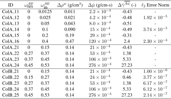
Two different types of non-dilute displacement experiments were conducted. For experimental set 1, pure water was the resident fluid and was displaced by solutions containing varying amounts of CaBr2. With experimental set 2, the mass fraction of CaBr2 in the displacing and displaced fluids was varied so that the density difference between the two fluids was the same for each experiment. Exper-imental sets 1 and 2 were performed in Column A and only experExper-imental set 2 was run in Column B. Table 2.1 shows the fluid properties of the incoming and resident fluids for the experiments. For the tracer and non-dilute displacement experiments, the minimum percent mass recovered was 99.93%, which is consistent with the accuracy of the density meter. The naming convention for the experiments first specifies which column was used, the experimental set, and finally the experiment number. The mass fraction of the CaBr2of the displacing fluid increased for each experimental number and T repre-sents a tracer study.
Table 2.1: Experimental conditions for displacement experiments showing the difference in the fluid properties between the displacing and displaced fluids.
ID ωAwres ωAwin ∆ρw(g/cm3) ∆ˆµ(g/cm-s) ∆ˆγAw(-) `2Error Norm
ColA 11 0 0.0125 0.011 2.2×10⁻⁴ -0.43
-ColA 12 0 0.025 0.021 4.2×10⁻⁴ -0.48 1.92×10⁻⁵
ColA 13 0 0.05 0.043 8.0×10⁻⁴ -0.51
-ColA 14 0 0.1 0.090 15×10−4 -0.49 3.74×10⁻⁵
ColA 15 0 0.2 0.19 29×10−4 -0.31
-ColA 16 0 0.4 0.47 120×10−4 2.4 2.30×10⁻⁴
ColA 21 0 0.15 0.14 21×10−4 -0.43
-ColA 22 0.27 0.37 0.14 53×10−4 1.38
-ColA 23 0.37 0.45 0.14 106×10−4 5.33
-ColA 24 0.45 0.53 0.14 276×10−4 27.23
-ColB 21 0 0.15 0.14 21×10−4 -0.43 1.00×10⁻⁶
ColB 22 0.15 0.27 0.14 24×10−4 0.46 3.77×10⁻⁷
ColB 23 0.27 0.37 0.14 53×10−4 1.38 6.17×10⁻⁷
ColB 24 0.37 0.45 0.14 106×10−4 5.33 6.12×10⁻⁷
ColB 25 0.45 0.53 0.14 276×10−4 27.23 2.14×10⁻⁷
to 0.5 when one pore volume of displacing fluid was pumped into the system, where one pore vol-ume is equal to the total volvol-ume of water in the column. Due to fluctuations in the pumping rate and errors in the time measurements, this was not observed. To correct the phase error, a time correction parameter was applied to match the assumed condition; these corrections were typically small and well within the expected experimental error. Once the phase error was removed, the outflow mass frac-tion of CaBr2was splined for the duplicate experiment so that the data could be compared at identical times. The`2error norm was then calculated at each time step and normalized by the number of data points. The error norms for the experiments in Column B were at least an order of magnitude lower for each duplicate experiment than for Column A. The columns were reused for many experiments. The fitted tracer dispersivities for Column A changed more than Column B, which is consistent with the experimental error norms and is a result of minor changes in pore structure with time. No changes in the experimental set-up or procedure changed between the two columns. The error norms for the duplicate experiments provide a bound on the accuracy that would be expected from an ideal model and provides a means to evaluate model error versus experimental error.
2.5.3 Dilute Flow and Transport
The laboratory experiments were modeled as a one-dimensional system, therefore, only the lon-gitudinal dispersivity coefficient needed to be fit to the dilute experiments to fully parameterize the dispersion. The dilute flow and transport model was used to determine the longitudinal dispersivity for the four dilute experiments that were performed.
For the parameter estimation, the`2 error norm between the observed outflow mass fraction from the model and the laboratory experiments was minimized. A time correction parameter was fit to the data to adjust for any phase error, which was previously discussed. Phase error in the experimental results stemmed from time measurement errors, and variations in tubing lengths and flow rates. The optimized longitudinal dispersivity values and time correction factors for the four tracer experiments are included in Table 2.2. The time correction parameters were within expected error bounds and small compared to the duration of the experiments, where 15,400 seconds were required for one pore volume of fluid to pass through column A and 15,200 seconds for column B. For the non-dilute simulations, the optimized longitudinal dispersivity value of the tracer experiment that preceded the experiment was used.
Table 2.2: Fitted Longitudinal Dispersivity Experiment αˆL(cm) tcorr (s)
Col AT1 0.137 -40.7
Col AT2 0.155 -42.7
Col BT1 0.108 -19.1
Col BT2 0.098 -11.7
outflow profile is asymmetric according to our laboratory data. For the sharpest experiment, the fitted dispersion coefficient approaches the effective molecular diffusion coefficient of 0.096×10⁻⁴ cm/s2. It can be observed from these two cases that non-dilute transport can result in marked sharpening of a breakthrough curve compared to an ideal dilute tracer.
● ● ● ● ● ● ● ● ● ● ● ● ● ● ● ● ● ● ● ● ● ● ● ● ● ● ● ● ● ● ● ● ● ●
0.8 0.9 1.0 1.1 1.2
0.0 0.2 0.4 0.6 0.8 1.0
Pore Volumes
Nor
maliz
ed Mass Fr
action
●●●●●●●●●●●●●●●●●●●●●●●●●●●●●●●●●●●●●●●●●●●●●● ●●●●●● ● ● ● ● ● ● ● ● ● ● ● ● ● ● ● ● ● ● ● ● ● ● ● ● ● ● ● ● ●● ●●●● ●●●●● ●●●●●●●●●●●●●●●●●●●●●●●●●●●●●●●●●●●●●●●●●●●●●●●●●●●●●●●●●●●●●●●●●●●●●●●●●●●●●●●●●●●●●●●●●●●●●●●●●●●●●● ● ● ColA_T2 Data ColA_T2 Model ColA_16 Data ColA_16 ModelFigure 2.1: Results from fitting the Fickian dispersion coefficient with the dilute flow and transport model for the least and most disperse scenarios. The least disperse experiment had an incoming CaBr2 mass fraction of 0.4 and pure water as the resident fluid.
2.5.4 Non-Dilute Parameter Estimation Results
The unknown parameters in the nonlinear Fickian and TCAT models, as well as time correction parameters, were fit by selecting a subset of the experimental data that was representative of the entire dataset. This was done for both of the columns as the packing of the porous media changed slightly between the two columns.