Zhang_unc_0153D_15904.pdf

BIOINFORMATICS TOOLS FOR EXPLORING REGULATORY MECHANISMS

Guosheng Zhang

A dissertation submitted to the faculty at the University of North Carolina at Chapel Hill in partial fulfillment of the requirements for the degree of Doctor of Philosophy in the

Curriculum in Bioinformatics and Computational Biology in the School of Medicine.

Chapel Hill 2016

Approved by: David Neil Hayes Leslie Lange Yun Li

ABSTRACT

Guosheng Zhang: Bioinformatics Tools for Exploring Regulatory Mechanisms (Under the direction of Yun Li)

Gene expression is the fundamental initial step in the flow of genetic information in biological systems and it is controlled by multiple precisely coordinated regulatory mechanisms, such as structural and epigenetic regulations. Dysregulation of gene expression plays important roles in the development of a broad range of diseases. Modern high-throughput technologies provide unprecedented opportunities to investigate these diverse regulatory mechanisms on a genome-wide scale. Here we develop several methods to analyze these omics profiles.

First, Hi-C experiments generate genome-wide contact frequencies between pairs of loci by sequencing DNA segments ligated from loci in close spatial proximity. To detect biologically meaningful interactions between loci, we propose a hidden Markov random field (HMRF) based Bayesian method to rigorously model interaction probabilities in the two-dimensional space based on the contact frequency matrix. By borrowing information from neighboring loci pairs, our method demonstrates superior reproducibility and statistical power in both simulation studies and real data analysis.

and our method showed higher imputation accuracy. The simulated association study further demonstrated that our method substantially improves the statistical power to identify trait-associated methylation loci in epigenome-wide association study (EWAS).

To my family and friend, I couldn’t have done this without you. Thank you for all of your support along the way.

ACKNOWLEDGEMENTS

First of all I would like to offer countless thanks to my adviser, Dr. Yun Li, for her tireless support and encouragement, and each of my committee members Wei Sun, David Neil Hayes, Karen Mohlke and Leslie Lange for their thoughtful contributions to this research. I would also like to thank my collaborators from UNC-Chapel Hill and other organizations for their invaluable comments and suggestions: Ming Hu from New York University Department of Population Health; Jian Kang from University of Michigan Department of Biostatistics; Fulai Jin for sharing the Hi-C data used in chapter 3; Karen N. Conneely for providing the DNA

TABLE OF CONTENTS

LIST OF TABLES ... x

LIST OF FIGURES ... xi

LIST OF ABBREVIATIONS ... xiii

CHAPTER 1 MOTIVATION AND BIOLOGICAL JUSTIFICATION ... 1

1.1 Gene Expression and Regulation ... 1

1.2 Chromosome Structure ... 2

1.3 Somatic Copy Number Aberration ... 3

1.4 DNA Methylation ... 3

CHAPTER 2 LITERATURE REVIEW ... 6

2.1 Early Methods for 3C-based Data Analysis ... 6

2.2 Early Methods for DNA Methylation Imputation ... 8

2.3 Early Methods for Integrative Analysis ... 10

CHAPTER 3 A BAYESIAN MODEL FOR THE DETECTION OF LONG- RANGE CHROMOSOMAL INTERACTIONS IN HI-C DATA ... 13

3.1 Introduction ... 13

3.2 Methods ... 15

3.2.1 Notations ... 15

3.2.2 Mixture of Negative Binomials ... 15

3.2.4 Bayesian Inference and the Joint Probability ... 18

3.3 Results ... 19

3.4 Discussion ... 32

CHAPTER 4 ACROSS-PLATFORM IMPUTATION OF DNA METHYLATION ... 36

4.1 Introduction ... 36

4.2 Materials and Methods ... 37

4.2.1 Data ... 37

4.2.2 Penalized Functional Regression Model ... 39

4.2.3 Selection of Local Covariates ... 42

4.2.4 Quality Filter ... 42

4.2.5 Imputation Quality Assessment ... 43

4.2.6 Simulation of Association Study ... 44

4.3 Results ... 45

4.3.1 Evaluation of Imputation Quality ... 45

4.3.2 Performance of Quality Metrics ... 50

4.3.3 Power Gain in Association Study ... 53

4.4 Discussion ... 55

CHAPTER 5 INTEGRATIVE ANALYSIS OF INFLAMMATION-RELATED GENES IN HBV-RELATED HEPATOCELLULAR CARCINOMA ... 60

5.1 Introduction ... 60

5.2 Materials and Methods ... 61

5.2.3 Array-based Data Production ... 63

5.2.4 Array-based Data Analysis ... 64

5.2.5 Validation Using Public Dataset ... 65

5.2.6 Validation in the Independent Sample ... 65

5.2.7 Gene Network Construction ... 66

5.3 Results ... 66

5.3.1 Identification of Aberrant Expression, Methylation and SCNA in Inflammation-related Genes ... 67

5.3.2 Contribution of Methylation and SCNA to Aberrant Expression of Inflammation-related Genes ... 69

5.3.3 Validation of Methylation and SCNA Relevant to Aberrant Inflammation-related Gene Expression ... 71

5.3.4 Functional Network Construction ... 74

5.4 Discussion ... 76

CHAPTER 6 CONCLUDING REMARKS ... 80

LIST OF TABLES

Table 3.1 Genome-wide real data evaluation based on False Positive

Rate (FPR), False Discovery Rate (FDR) and Recover Rate (RR) ... 21

Table 3.2 Genome-wide real data evaluation based on the consistency measure ... 22

Table 4.1 Quantiles of imputation MSE and R2 ... 47

Table 4.2 Number of probes passing post-imputation quality filter ... 52

Table 4.3 Imputation quality of SNP-probes versus non-SNP-probes ... 58

Table 5.1 Clinical characteristics of 30 HCC patients with array data and 47 patients with validation data ... 62

LIST OF FIGURES

Figure 3.1 Overlapping histograms of inverse temperature 𝜓 estimates

in combined, before and after TNF-α treatment ... 18

Figure 3.2 Peaks called in the domain Chr.17:29.52Mb-29.72Mb ... 20

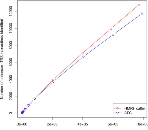
Figure 3.3 Power to identify enhancer-TSS interactions ... 25

Figure 3.4 CTSB, potential target gene for GWAS variant rs1600249 ... 26

Figure 3.5 TFBS and active-TSS enrichment ... 28

Figure 3.6 Transcription factor binding site (TFBS) enrichment analysis, at fragment level ... 29

Figure 3.7 Active transcription starting site (TSS) enrichment analysis, at fragment level ... 30

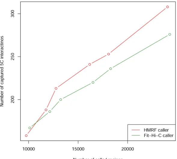
Figure 3.8 Power to detect interactions captured by hESC 5C dataset ... 31

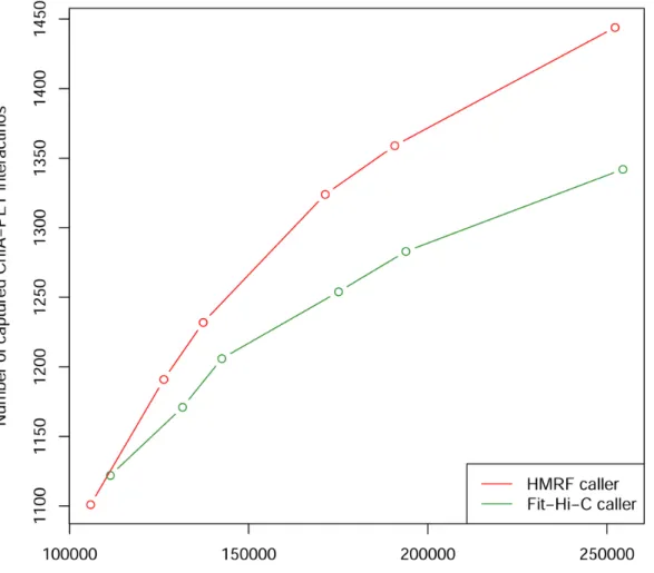
Figure 3.9 Power to detect interactions captured by mESC ChIA-PET dataset ... 32

Figure 4.1 Empirical cumulative density function of imputation MSE for different Kb values ... 41

Figure 4.2 Empirical cumulative density function of imputation R2 for different Kb values ... 42

Figure 4.3 Empirical cumulative density function of imputation MSE for probes showing large variations in the AML dataset ... 46

Figure 4.4 Empirical cumulative density function of imputation R2 for probes showing large variations in the AML dataset ... 47

Figure 4.5 Methylation profiles of a North Shelf probe cg00288598 and 10 selected local probes ... 49

Figure 4.6 The individual-specific density plot of methylation values from all HM27 probes in North Shelf regions ... 50

Figure 4.7 Scatter plot of under-dispersion measure and imputation MSE ... 51

continuous trait across a spectrum of effect size c ... 54 Figure 4.10 Empirical power of simulated association tests for binary

trait across a spectrum of effect size c ... 55 Figure 5.1 Identification of inflammation-related genes exhibiting

coordinative changes between mRNA expression and DNA

methylation or SCNA in HBV-related HCCs ... 68

Figure 5.2 Relationship between mRNA expression and DNA methylation

or SCNA of the randomly selected inflammation-related genes ... 70

Figure 5.3 Venn diagram of the overlapping inflammation-related genes having significant mRNA expression, or DNA methylation in HBV-related

HCCs in our study with public datasets ... 72

Figure 5.4 Validation of mRNA expression, DNA methylation and copy number variation of the randomly selected inflammation-related

genes in 47 samples ... 73

Figure 5.5 The functional network of top inflammation-related genes created by integrative analysis of mRNA expression associated with

LIST OF ABBREVIATIONS

AFC AML

Anchor-Fragment Caller Acute Myeloid Leukemia CCLE CGI CNV DNMT ENCODE ESC EWAS

Cancer Cell Line Encyclopedia CpG Island

Copy Number Variation DNA Methyltransferases

Encyclopedia of DNA Elements Embryonic Stem Cell

Epigenome-wide Association Study FDR FPR GEO GWAS HBV HCC HCV HM27 HM450 HMM HMRF

False Discovery Rate False Positive Rate

Gene Expression Omnibus Genome-wide Association Study Hepatitis B Virus

Hepatocellular Carcinoma Hepatitis C Virus

Illumina HumanMethylation27 BeadChip Illumina HumanMethylation450 BeadChip Hidden Markov Model

Hidden Markov Random Field LD

LOESS

Linkage Disequilibrium

LRR MSE PCR PLS QC RR SCNA

Log R Ratio

Mean Squared Error

Polymerase Chain Reaction Partial Least Squares Quality Control Recovery Rate

Somatic Copy Number Aberration SNP

SVM TAD

Single Nucleotide Polymorphism Support Vector Machine

Topologically Associating Domain

TCGA The Cancer Genome Atlas

TFBS Transcription Factor Binding Site TNF

TSS

CHAPTER 1 MOTIVATION AND BIOLOGICAL JUSTIFICATION

In this document, we will discuss bioinformatics methods for exploring various

regulatory mechanisms of gene expression. This section provides an overview of the biological problems we are interested in.

1.1 Gene Expression and Regulation

Gene expression is fundamental in the process by which static DNA information

translates into dynamic phenotypes. Understanding gene expression is essential for interpreting functional elements in the genome, identifying molecular systems in cells, and understanding the developmental process. The gene expression programs that establish specific cell states during cell differentiation are controlled by multiple regulatory mechanisms. Dysregulation of these gene expression programs plays important roles in the development of a broad range of diseases.

three types of regulations, chromosome structure, somatic copy number aberrations and DNA methylation.

1.2 Chromosome Structure

Chromosomal DNA must be packed nearly three orders of magnitude to fit within the limited space of the nucleus. The intricate, highly compacted folding of the chromosomes, however, is by no means random. Recent technological advances have made it possible to delineate the three-dimensional (3D) organization of the genome [de Wit and de Laat 2012]. It is becoming increasing clear that chromatin architectures are intimately linked to transcription regulation by influencing how genetic information is accessed, read, and interpreted in a given cell and under certain micro-environmental conditions via dynamic interactions among genes and their regulatory elements [Splinter and de Laat 2011].

One prominent feature of the genome is the formation of chromosomal domains at multiple scales [Gibcus and Dekker 2013]. At ~1-10Mb scale, compartments of transcriptionally active euchromatin and inactive heterochromatin are spatially segregated [Lieberman-Aiden, et al. 2009; Simonis, et al. 2006]. Recently, the genome was further shown to be subdivided into conserved topologically associating domains (TADs) at the subcompartment level, which can be hundreds of kilobases in size [Dixon, et al. 2012; Nora, et al. 2012]. A specific locus tends to interact much more frequently with loci located within the same TAD, compared to loci located outside its TAD. The boundaries between TADs are genetically encoded, which was

2009]. Within TAD, a long-range loop structure can be formed to link a distant enhancer with its target gene to regulate gene transcription. Hence, characterization of the 3D genome

organizations is critical to understanding how the chromatin structure influences cell fate determination during development [Dekker, et al. 2013; Sajan and Hawkins 2012].

1.3 Somatic Copy Number Aberration

Cancer genesis and progression are enabled through the stepwise accumulation of

genomic alterations in somatic cells, including point mutations, somatic copy number aberrations (SCNA), and fusion events, that affect the function of critical genes regulating cell proliferation and apoptosis [Hanahan and Weinberg 2011]. Recurrent genomic abnormalities provide a selection advantage by targeting genes vital for tumorigenesis and metastasis [Albertson, et al. 2003]. Discovery and functional assessment of oncogenes and tumor suppressor genes being targeted by these abnormalities has spurred both the understanding of tumorigenesis and the identification of novel therapeutic targets [Stratton, et al. 2009]. Genes targeted by SCNA, in particular, play central roles in oncogenesis as SCNA results in altered expression of these genes (dosage effect) [Santarius, et al. 2010]. A recent work studied patterns of SCNA across 26 cancer types, and found 24 gains and 18 losses on average per tumor sample [Albertson, et al. 2003]. A literature review reveals numerous examples of genes identified as targets of focal or

chromosomal arm-level amplification or deletions. Most notable examples include amplified oncogenes ERBB2 [Slamon, et al. 1989], MYC [Alitalo, et al. 1983], CAD [Schimke, et al. 1978; Wahl, et al. 1979], BCR-ABL [Koivisto, et al. 1997] and AR [Gorre, et al. 2001], and deleted tumor suppressor genes PTEN [Li, et al. 1997], CDKN2A [Orlow, et al. 1995], RB1, BRCA1,

Epigenetic modifications are non-sequence changes in chromatin that inherited through cell division, which are often dynamic and tissue-specific [Cedar and Bergman 2012; Scarano, et al. 2005]. DNA methylation is an important epigenetic marker involved not only in normal development [Smith and Meissner 2013] but also in risk and progression to many diseases [Bergman and Cedar 2013]. DNA methylation is a process by which a methyl group is added to the cytosine residue. DNA methylation typically occurs in the context of CpG dinucleotide in the genome and it is mediated by DNA methyltransferases (DNMTs). It has been shown to play a key role in the regulation of gene transcription, X-inactivation, cellular differentiation, and other critical processes such as aging [Bird 2002; Gonzalo 2010].

genome, DNA methylation levels have been shown to be correlated with chromatin

modifications such as histone methylation [Hawkins, et al. 2010; Meissner, et al. 2008; Weber, et al. 2007], cis-regulatory elements, and proximal sequence pattern [Das, et al. 2006; Shen, et al. 2007], indicating the interaction between DNA methylation and cellular phenotypes.

CHAPTER 2 LITERATURE REVIEW

This section presents a partial review of many of the papers previously published on the topic of methods to study regulatory mechanisms. It is by no means complete since the number of these papers is quite large; however, it is an attempt to show the development of methods used to tackle these problems.

2.1 Early Methods for 3C-based Data Analysis

Recent advancements in chromosome conformation capture (3C) [Dekker, et al. 2002] and derived methods (such as 3C, 4C, 5C and Hi-C) allow the study of 3D chromosome organization with increasing resolution and throughput. These 3C-based methods quantify the interaction or contact frequency, how often any pair of loci in the genome is in close spatial proximity. For 3C, a locus is the unit of analysis and corresponds to one restriction enzyme fragment (hereafter termed fragment). Approaches to analyze interaction frequencies fall largely into two

This section focuses on peak calling. Several computational and statistical methods have been developed for this important peak calling task for data generated from 3C-based methods. Sanyal et al. [Sanyal, et al. 2012] developed a 5C peak calling algorithm where they first estimated the null contact frequencies (average and standard deviation) using nonparametric lowess smoothing over genomic distance (using all pairs with the assumption that the vast majority of interactions are random collisions), then calculated standardized z-scores and raw values by fitting the z-scores to a Weibull distribution, followed finally by converting the raw p-values into q-p-values for FDR analysis. Duan et al. [Duan, et al. 2010] binned pairs of loci according to genomic distance, estimated null contact probabilities within each bin, and called peaks by assuming the contact frequency of every pair in each bin followed an identical binomial distribution. Jin et al. [Jin, et al. 2013] developed a pipeline to estimate the expected contact frequency accounting for locus length, inter-locus distance, mappability, and GC content, and then tested for significant interaction by assuming the observed contact frequency followed a negative binomial distribution. Most recently, Ay et al. [Ay, et al. 2014] refined the binning method in Duan et al. [Duan, et al. 2010] and to develop Fit-Hi-C. Specifically, Fit-Hi-C provided more accurate estimates of the contact probabilities by fitting nonparametric spline curves across genomic distances (instead of discrete binning), re-fitting spline curves after filtering non-random collisions based on the initial spline, and modeling other Hi-C biases by incorporating locus-specific correction factors inferred from a previously published iterative correction and eigenvector decomposition method [Imakaev, et al. 2012].

estimation, with some [Ay, et al. 2014; Jin, et al. 2013] incorporating other genomic biases. However, all existing methods, by testing each individual pair of loci independently, ignore the potential correlation among pairs of loci. This was less of an issue with lower resolution data when multiple fragments combined into meta-fragments served as the units of analysis.

When analyzing a fragment resolution Hi-C data, Jin et al. [Jin, et al. 2013] recognized this potential issue and developed the anchor-fragment caller (AFC), an ad hoc approach to accommodate the correlation of peak status among neighboring fragment pairs. In AFC, one anchor was fixed (either a fragment or mega-fragment from consecutive smaller fragments) and one-dimensional peak calling was performed. For each anchor, the algorithm started with the identification of candidate peak regions. A candidate peak region could encompass multiple consecutive fragments with moderate marginal evidence for non-random interaction with the anchor and, importantly, AFC allows for small gaps. Peaks were called by aggregating

information across the entire candidate peak region via assigning thresholds on read counts and p-values from contributing fragment pairs as well as from the entire region cumulatively. As an initial attempt to model the spatial dependency of the underlying peak status, AFC performed reasonably.

2.2 Early Methods for DNA Methylation Imputation

Most existing methods formulate the methylation prediction as a binary classification problem, i.e., distinguish between methylated and unmethylated CpG sites [Fan, et al. 2008; Fang, et al. 2006]. Related methods conduct methylation imputation at two levels – CGI (or CpG-rich region) or CpG dinucleotide. At the CGI level, average methylation status for windows of the genome is predicted, and some studies achieve a > 90% accuracy. However, as we

mentioned earlier, most CpG sites residing within CGIs tend to remain unmethylated across the whole genome [Jones 2012]. Thus it is not surprising that these methods can achieve a high accuracy in these regions. At the CpG dinucleotide level, methylation status is predicted for individual CpG sites, and usually the accuracy is lower [Bhasin, et al. 2005]. A few studies predict methylation levels as a continuous variable, but instead of genome-wide analysis, the prediction is limited to specific genomic regions.

A key step for building these predictive models is to select features. The features can be roughly grouped into two categories: genetic and epigenetic. Genetic features include (1) proximal DNA sequence patterns, (2) distribution patterns of functional and evolutionarily conserved elements [Siepel, et al. 2005], such as transcription factor binding sites (TFBSs), (3) DNA structure (e.g., co-localized introns), (4) GC contents, and (5) functional annotation of nearby genes. Epigenetic features mainly include methylation and acetylation status of the

histones. Several studies used only DNA composition [Bhasin, et al. 2005; Das, et al. 2006; Zhou, et al. 2012], or methylation levels of the same CpG sites from different tissues as features [Ma, et al. 2014], while some used several hundred features, including DNA composition, DNA

The majority of these methods are based on support vector machine (SVM) classifiers using linear kernel [Bhasin, et al. 2005; Bock, et al. 2006; Das, et al. 2006; Fan, et al. 2008; Fang, et al. 2006; Ma, et al. 2014; Previti, et al. 2009; Zheng, et al. 2013; Zhou, et al. 2012], where non-additive interactions between features are not modeled. Several studies found that decision tree [Previti, et al. 2009], random forest [Zhang, et al. 2015], or naïve Bayes classifier can achieve better prediction performance.

2.3 Early Methods for Integrative Analysis

Biological system is subjected to precisely coordinated controls at multiple layers, across the levels of genetic, epigenetic, transcriptional, and translational regulations. Different layers intertwined to form multiple complex and extensively coupled networks [Maniatis and Reed 2002; Moore 2005; Orphanides and Reinberg 2002]. Recent development of various

high-throughput technologies has enabled researchers to collect diverse information on the same set of samples. Microarray and next-generation sequencing technologies are used to profile genome-wide gene expression levels, genetic variations (e.g. SNP and CNV), epigenetic regulation (e.g. DNA methylation and histone modifications), post-transcriptional regulation (e.g. microRNA expression), and protein abundance. The amount of available biological data from multiple technologies and platforms is expanding rapidly. Large online databases such as the UCSC Genome Browser [Speir, et al. 2016] and large-scale projects such as The Cancer Genome Atlas (TCGA) [Cancer Genome Atlas Research 2008] often contain multiple data types collected from a cohort of samples.

these different regulatory layers. Since different data types have different scales and units, we cannot simply combine them for analysis, thus novel computational methods are needed to explore associations among multiple data types and aggregate these multiple data sources when making inference about the samples.

Earlier relevant efforts focused on analyzing two-dimensional genomic datasets. For example, eQTL method can jointly analyze SNP and gene expression data to identify target genes of regulatory SNPs [Zhang, et al. 2010]. General methods such as partial least squares (PLS) were also used to examine the relation between two sets of variables. However, the restriction of these methods to pairwise comparisons limits its utility in examining relations among more than two data types. Recently, several methods have been developed to analyze genomic datasets with more than two data types. For example, multiple canonical correlation analysis (mCCA) was introduced as an extension of PLS to more than two data types [Witten and Tibshirani 2009], and it can explore associations and structures on multi-omics data in a supervised manner. Several unsupervised methods were also proposed. For example, iCluster incorporates a joint latent variable model for integrative clustering and tumor subtype discovery [Shen, et al. 2009]. An adaptive clustering approach was also developed to integratively analyze genome-wide gene expression, DNA methylation, microRNA expression, and copy number alteration profiles [Zhang, et al. 2013a].

CHAPTER 3 A BAYESIAN MODEL FOR THE DETECTION OF LONG-RANGE

CHROMOSOMAL INTERACTIONS IN HI-C DATA

3.1 Introduction

Identifying non-random contacts in the 3D genome organization is of fundamental biological interest to researchers due to their relevance for functional regulation. For instance, it can shed light on the functional mechanisms of non-coding complex trait associations identified in genome-wide association studies (GWAS). GWAS have been resoundingly successful, identifying thousands of variants associated with complex traits. However, only a small proportion (7~12%) fall in protein coding regions [Hindorff, et al. 2009; Kumar, et al. 2012; Pennisi 2011; Ward and Kellis 2012], making interpretation of non-coding variants imperative. Although a large number of regulatory elements have been annotated [Consortium 2012; Maurano, et al. 2012], their target genes are largely unknown [Jin, et al. 2013; Niu, et al. 2014]. Recent 3C-based studies are generating an increasingly comprehensive catalog of interactions between genes and their regulatory elements in different cell types at varying resolution across multiple organisms including drosophila, yeast, mouse, and human [Hou, et al. 2012; Lieberman-Aiden, et al. 2009; Sexton, et al. 2012; Smallwood and Ren 2013]. Such information will be fundamental to understanding functional mechanisms. For example, a recent study [Smemo, et al. 2014] used 4C data to identify long-range (at megabase distances) interactions between the

obesity-associated intronic variants in FTO and the homeobox gene IRX3, with the expression of

interactions identified from the 3C-based studies for shedding light on the functional mechanisms of genetic variants implicated by GWAS.

Several computational and statistical methods have been developed for peak calling for data generated from 3C-based methods. However, we believe that the existing methods are not yet optimal, and that improvements in multiple aspects are needed. First, an improved analysis suite for data from 3C-derived methods should be based on an explicit model that yields clear and reproducible expectations for genome-wide interaction frequencies. Second, existing approaches choose anchor fragment(s) arbitrarily and also ignore any correlations between neighboring fragments or anchors. For example, we found that neighboring anchors often

interact with the same target fragments, suggesting that these anchors are parts of a bigger region involved in the same DNA looping event. Therefore an ideal peak caller should consider

correlations between neighboring fragments in the context of a two-dimensional (2D) contact matrix generated from 3C-derived technologies. Third, one-dimensional calling approaches are not optimal, do not incorporate useful existing information, and considerable benefits can be gained using a 2D approach. For example, we observed AFC asymmetric peak calls and lower power in the identification of non-random interactions (details in Results section). Thus, these observations motivated us to develop rigorous statistical models that efficiently use information from neighbors in the 2D space.

3.2 Methods

3.2.1 Notations

Hi-C generates a contact frequency matrix between pairs of fragments. Assume a total of

𝑁 fragments under consideration. Let 𝑢_!", 1≤𝑖 <𝑗 ≤𝑁 denote the observed contact frequency

between fragment 𝑖 and fragment 𝑗. Similarly, let 𝑒_!", 1≤𝑖 <𝑗 ≤𝑁denote the expected contact

frequency between fragment 𝑖 and fragment𝑗 under random collisions. Let the binary indicator variable 𝑍_!" take two possible values 1 and −1 which represent the peak status underlying

fragment pair 𝑖 and 𝑗, with 𝑍_!" = 1 corresponding to a peak (i.e., a non-random interaction) and

𝑍!" =−1 corresponding a non-peak (i.e., a random collision event).

3.2.2 Mixture of Negative Binomials

We assume that the observed contact frequencies 𝑢!" follow a negative binomial

distribution, 𝑢_!"~𝑁𝐵 𝜇_!",𝜙 , where 𝜙is the over-dispersion parameter and 𝑢_!" has mean 𝜇_!" and

variance 𝜇_!" +𝜇_!"!_{/𝜙. The benefit of using a negative binomial distribution (over Poisson or}

binomial distribution) is its allowance for over-dispersion, often observed in Hi-C data [Jin, et al. 2013].

Furthermore, we assume that the observed contact frequencies follow a mixture of negative binomial distributions as a consequence of the mixture of underlying interaction status

𝑍_!"’s. Specifically, let 𝜃 >0 represent the peak to background ratio (signal to noise ratio). We

assume the following on 𝑙𝑜𝑔𝜇!":

𝑙𝑜𝑔𝜇!" =

𝑙𝑜𝑔𝑒!"+𝜃, 𝑍!" =1

where 𝑒_!"’s are expected counts under random collision events, estimated using existing methods

such as ICE [Imakaev, et al. 2012] or Fit-Hi-C [Ay, et al. 2014]. Thus we use the following negative binomial mixture distribution:

𝑢_!"~𝑁𝐵 𝑒_!"𝑒!(!!"!!)/!,𝜙 .

3.2.3 Hidden Markov Random Field (HMRF) Model

A HMRF is a generalized hidden Markov model (HMM) in a higher dimensional space [Besag, et al. 1995]. Instead of an underlying Markov chain in HMM, HMRF has an underlying Markov random field, a set of random variables having a Markov property described by an undirected graph. HMRF has been applied in genetics, including evaluation of population structure [François, et al. 2006], gene expression data [Stingo and Vannucci 2011], network-based genomic discovery [Wei and Pan 2010], and GWAS [Li, et al. 2010]. We use HMRF to account for the local spatial dependency among adjacent fragment pairs, and simultaneously detect all 2D peaks by borrowing information from neighboring fragment pairs. Our HMRF modeling is conceptually similar to the employment of HMM or Bayesian hidden Ising model for peak identification from ChIP-Seq data [Choi, et al. 2010; Mo 2012; Qin, et al. 2010], but we extend the modeling from a one-dimensional space to a two-dimensional space. In our HMRF model, we adopt the following Ising prior [Kindermann, et al. 1980] for the binary variable 𝑍_!" ∈ −1,1 representing the unobserved peak status underlying fragment 𝑖 and fragment 𝑗 such

that 𝑍!! only depends on the status of four neighboring fragment pairs 𝑖+1,𝑗 , (𝑖−1,𝑗),

(𝑖,𝑗+1) and (𝑖,𝑗−1):

𝜋 𝑍_!"|𝜓 = exp 𝜓𝑍!" !!!!!!!!!!!𝑍!!!!

where 𝜓 is the inverse temperature parameter measuring the level of clustering among 𝑍_!"’s. The

term 𝑊(𝜓) is the normalizing function ensuring the probability mass sum to 1. The case 𝜓=0 corresponds to independent uniform prior on 𝑍_!"’s, analogous to the disordered states at infinite

temperature. Large values of 𝜓 correspond to more tightly clustered configurations of 𝑍_!"’s,

analogous to more ordered/correlated states at low temperature. In Hi-C data, positive clustering is expected, particularly with the high-resolution Hi-C data where neighboring fragment pairs are likely to share the underlying peak or non-peak status. Our model explicitly models the level of clustering and estimates the value of 𝜓 based on data [Besag, et al. 1995]. Although our model is

Figure 3.1 Overlapping histograms of inverse temperature 𝜓 estimates in combined (gray), before (blue) and after (red) TNF-α treatment.

3.2.4 Bayesian Inference and the Joint Probability

We adopt a Bayesian approach [Gelman 2004] for parameter inference where the inference is based on the posterior distributions. We will start with specifying the priors. For convenience and computational efficiency, we make a re-parameterization: 𝛾 =𝜙!!_{. By default, our model}

uses weak priors with large variance: a translated gamma distribution for 𝜃 :

𝜋 𝜃 =𝐺𝑎𝑚𝑚𝑎(𝜃−𝜃!;2,2), a gamma distribution for γ: γ~𝐺𝑎𝑚𝑚𝑎(γ;0.1,1) and a uniform

𝜃_! is fixed to ensure model identifiability (we use 𝜃_! =0.5 by default). The likelihood is fully

specified based on the mixture of negative binomial distributions introduced earlier. Combined with the conditional independence assumption of 𝑢_!" given 𝑍_!", we have

𝜋 𝑢!" 𝑍!" ,𝜃,𝛾 =

1

𝛾

1

𝛾+𝑒!"𝑒!(!!"!!)/! ! !

Γ 1_𝛾+𝑢_!"

Γ 1_𝛾 𝑢_!"! !!!!!!!

𝑒!"𝑒!(!!"!!)/! 1

𝛾+𝑒!"𝑒!(!!"!!)/!

!!"

.

The posterior probability can be written as

𝜋 𝑍_!" ,𝜃,𝛾,𝜓| 𝑢_!" ∝𝜋 𝑢_!" , 𝑍_!" ,𝜃,𝛾,𝜓 =𝜋 𝑢_!" 𝑍_!" ,𝜃,𝛾 𝜋 𝑍_!" |𝜓 𝜋 𝜃 π 𝛾 π 𝜓 .

We used Metropolis-Hastings algorithm to infer all parameters except the inverse temperature parameter 𝜓, which is estimated using a pseudo-likelihood approach.

3.3 Results

Comprehensive simulation studies have demonstrated the superior performance of our HMRF Bayesian caller over other available methods. In particular, our simulations showed that our model is able to accurately estimate the inverse temperature parameter 𝜓 across a wide range

patterns observed under each condition separately. Motivated by this finding and the insufficient sequencing depth in each condition (i.e., before or after TNF-α treatment), we combined data from the two conditions to achieve higher statistical power in detecting fragment resolution chromatin interaction.

Figure 3.2 Peaks called in the domain Chr.17:29.52Mb-29.72Mb. For each dataset (combined, before, and after TNF-𝜶 treatment), the same number of peaks as using AFC method was shown (based on posterior probabilities for HMRF and p-values for Fit-Hi-C) for comparison.

patterns of the two conditions are shared, a robust caller is expected to identify similar patterns for the three datasets. Figure 3.2 shows peak calling results from one domain chr17: 29.52Mb-29.72Mb. We observed that fewer peaks were called in datasets 1 and 2, particularly dataset 1 where the total number of reads was 75.1% of that in the dataset 2. Comparatively, our method encourages more clustering of peaks and more consistent results across the three datasets. For example, within this particular domain, 40.6% and 69.9% of the peaks called in the combined dataset were detected using only dataset 1 and 2, respectively, by our method, compared with 35.3% and 65.2% (40.3% and 67.9%) by AFC (Fit-Hi-C). Genome-wide quantitative

comparisons are presented below (Table 3.1 and Table 3.2).

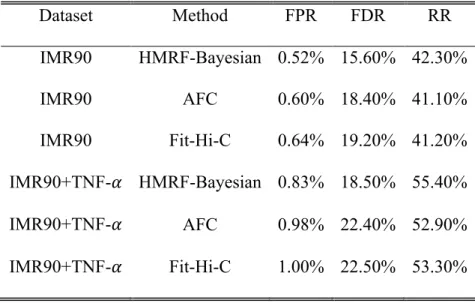
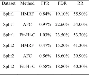
Table 3.1 Genome-wide real data evaluation based on False Positive Rate (FPR), False Discovery Rate (FDR) and Recover Rate (RR). Assuming calling result for the combined dataset is the true peak pattern, we summarized the following measures for 1,432 domains, i.e. genome-wide. We reported the genome-wide average of false positive rate (FPR), false

discovery rate (FDR) and recovery rate (RR) by the HMRF-Bayesian method, AFC method and Fit-Hi-C for both IMR90 before TNF-𝜶 treatment and IMR90 after TNF-𝜶 treatment. We found that the HMRF-Bayesian method has better performance than AFC method and Fit-Hi-C.

Dataset Method FPR FDR RR

IMR90 HMRF-Bayesian 0.52% 15.60% 42.30%

IMR90 AFC 0.60% 18.40% 41.10%

IMR90 Fit-Hi-C 0.64% 19.20% 41.20%

IMR90+TNF-𝛼 HMRF-Bayesian 0.83% 18.50% 55.40%

IMR90+TNF-𝛼 AFC 0.98% 22.40% 52.90%

Dataset Method FPR FDR RR

Split1 HMRF 0.84% 19.10% 55.90%

Split1 AFC 0.97% 22.60% 54.00%

Split1 Fit-Hi-C 1.03% 23.50% 53.70%

Split2 HMRF 0.47% 15.20% 41.30%

Split2 AFC 0.56% 18.60% 39.90%

Split2 Fit-Hi-C 0.58% 18.80% 40.30%

Table 3.2 Genome-wide real data evaluation based on the consistency measure (Jaccard Index).

Method IMR90 vs. IMR90+TNF-α* Split1 vs Split2*

HMRF 22.1±0.33% 22.7%±0.32%

AFC 18.4±0.32% 18.5%±0.31%

Fit-Hi-C 13.7±0.29% 13.6%±0.28%

*Mean±SE

FP, TP, FN and TN, where the truth is defined according to AFC results from the combined dataset and the four numbers sum up to the total number of intra-domain fragment pairs. We have FPR=FP/(FP+TN), FDR=FP/(FP+TP), and RR=TP/(TP+TN). As shown in Table 3.1 upper panel, methods accounting for potential dependency of underlying peak statuses (AFC and our HMRF Bayesian caller) resulted in better performance than Fit-Hi-C which models fragment pairs independently. Furthermore, our method outperformed the others for all three measures. For example, for IMR90 before TNF-α treatment, we obtained FPR=0.52%, FDR=15.6% and

RR=42.3% for our HMRF Bayesian caller, compared with FPR=0.60%, FDR=18.4% and RR=41.1% for AFC, and FPR=0.64%, FDR=19.2% and RR=41.2% for Fit-Hi-C. By borrowing information from neighboring fragment pairs in a probabilistic framework, our method lead to more robust inference with simultaneously lower false positive, false discovery rates and higher recovery rate.

In addition, for each caller, we calculated the Jaccard Index [Hamers, et al. 1989] between the peak sets from the two conditions, defined as the ratio of number of peaks identified under both conditions over the number of peaks identified by either. Average Jaccard Index across all domains genome-wide is shown in Table 3.2 for each method. Again, methods accounting for the dependency of underlying peak status show higher concordance across conditions. Average Jaccard Index improved by 33.6% and 61.3% respectively, from 13.7% (Fit-Hi-C) to 18.4% (AFC) and 22.1% (HMRF).

Table 3.1 (lower panel) and Table 3.2 (rightmost column) similarly show better reproducibility and robustness of our methods over existing ones.

Figure 3.4 CTSB, potential target gene for GWAS variant rs1600249.

In addition, we performed transcription factor binding sites (TFBS) and active TSS (reported by Jin, et al., 2013) enrichment analysis to elucidate the biological relevance of identified interactions. Specifically, we evaluated two aspects. First, we tested if fragment pairs detected as interacting loci are enriched with TFBS. Second, we compared the number of interacting loci for TFBS versus non-TFBS. We used ENCODE IMR90 TFBS information retrieved from

detection threshold (ranging from 1 in 100,000 fragment pairs called as peaks to 1 in 100), the pairs of interacting fragments called are significantly enriched with TFBS and active TSS (χ!

p-value < 10!!"#_{) with ~42% identified peak pairs overlapping with TFBS while ~28% identified}

non-peak pairs overlapping with TFBS (Figure 3.5). In addition, we found that fragments overlapping with TFBS or active TSS are involved in a slightly (but statistically significant) larger number of interactions than those not overlapping with TFBS or active TSS (Figure 3.6 and Figure 3.7).

Figure 3.9 Power to detect interactions captured by mESC ChIA-PET dataset.

3.4 Discussion

nevertheless a prerequisite, not peak calling itself. None of the existing methods consider the dependency underlying the peak status with statistical rigor.

In this work, we propose a HMRF based Bayesian method that explicitly models the dependency of the underlying peak pattern. The true peak pattern is unknown and can take different forms in the presence of dependency. We simplify the problem by assuming an Ising distribution prior and learn the level of dependency from data in a Bayesian framework. Our extensive simulations indicate superior performance in terms of both the estimation of the extent of dependency and the statistical power to distinguish peaks from background, across a range of underlying dependency patterns.

There are several aspects where the model can be further elaborated. First, our model has one 𝜃, one 𝜓, and one 𝜙, thus assuming that peaks are of similar strength and clustering patterns,

takes ~13 minutes for a typical domain with 200 fragments and with parallel computing, genome-wide analysis can be easily accomplished within a few hours. In contrast, Fit-Hi-C and our R implementation of AFC take ~4 seconds and ~12 minutes, respectively. Therefore, for future work, computationally more efficient algorithms warrant consideration. We attempted to apply the iterative conditional mode algorithm [Li, et al. 2010], but observed unsatisfactory performance with weak peak signals (data not shown).

reasonable silver standard. For example, for the IMR90 cell lines, we compared against results from the combined dataset with the highest sequencing depth, for H1 hESC and mESC, we used results from independent technologies (5C and ChIA-PET respectively).

CHAPTER 4 ACROSS-PLATFORM IMPUTATION OF DNA METHYLATION

4.1 Introduction

Recently, the emergence of powerful technologies such as microarray-based DNA

methylation studies [Bibikova, et al. 2011] and whole-genome bisulfite sequencing [Harris, et al. 2010] has enabled the profiling of DNA methylation levels at high resolution. Numerous studies employed these high-throughput approaches to characterize changes in DNA methylation patterns and their corresponding tissue and disease-specific differentially methylated regions on a genome-wide scale [Berman, et al. 2012; Chen, et al. 2014; Horvath 2013; Varley, et al. 2013].

only expensive but also time-consuming [Cancer Genome Atlas Research 2013; Getz, et al. 2013; Koboldt, et al. 2012; Network 2012].

Imputation has been successfully employed in many genetic, genomic and epigenomic contexts [Donner, et al. 2012; Ernst and Kellis 2015; Jewett, et al. 2012; Li, et al. 2009; Zhang, et al. 2015]. However, no cross-platform imputation methods have been proposed for predicting methylation levels at unassayed CpG sites. On the other hand, for genotypes, imputation of untyped SNPs has become a standard procedure used both to resolve similar inconsistencies between genotyping arrays and to increase the resolution of genotype data collected in genome-wide association studies [Li, et al. 2009]. Here we propose the application of a similar concept to impute data in DNA methylation profiles from a subset of probes. Although DNA methylation does not exhibit as clear or strong a correlation structure as LD blocks among SNPs, we observe local correlation among neighboring probes similar as reported by others [Eckhardt, et al. 2006; Zhang, et al. 2015]. Importantly, we have found non-local correlations among probes falling into the same functional categories that have not been employed in the literature. Therefore we adopt a penalized functional regression model [Goldsmith, et al. 2011], which uses functional

predictors to capture these non-local correlations. Our study demonstrates that this model can impute an HM27 dataset into an HM450 dataset effectively and accurately, and using these imputed values can improve the statistical power of downstream epigenome-wide association study (EWAS).

4.2 Materials and Methods

4.2.1 Data

of tumor tissues from 194 patients with AML and is one of the largest methylation datasets from the TCGA project. All samples were evaluated using both HM27 and HM450. We transformed

the raw β values into M values, defined as M =log2[β/ (1−β)], as the M values better follow a

Gaussian distribution [Cancer Genome Atlas Research 2013]. Our goal is to impute the HM27 dataset into an HM450 dataset to get an expanded view of the epigenomic landscape. The dataset is publicly available at the TCGA data portal (https://tcga-data.nci.nih.gov/tcga/).

Since imputation of sporadic missing data is not the focus of this work, we removed all probes with at least one missing values for the sake of convenience. However, these missing values can be imputed by applying similar methods developed for gene expression profiles [Bo, et al. 2004; Kim, et al. 2005; Liew, et al. 2011; Troyanskaya, et al. 2001] to generate data without missing values. Additionally, we removed 743 probes designed in HM27 but not in HM450. In total, the HM27 dataset consisted of 20,794 probes passing TCGA quality control (QC) criteria [Ley, et al. 2013] and the HM450 dataset consisted of 393,152 QC+ probes. The latter set contained all 20,794 probes in HM27, leaving the remaining 373,358 as our potential imputation targets.

When training and using our model, we required data from HM450 and HM27, respectively. However, we noted that as HM27 and HM450 employ different biochemical methods to measure methylation levels, platform-specific effects might negatively impact

4.2.2 Penalized Functional Regression Model

We employed the penalized functional regression model [Goldsmith, et al. 2011] with minor modifications detailed below to quantify the relationship between DNA methylation from HM450 probes and DNA methylation density function estimated from HM27 probes together with other covariates. Specifically, assume for each target HM450 probe we have n observations

and for each sample i = 1, 2, …, n, we have data , where is the transformed

DNA methylation level at the target HM450 probe, is the sample specific density function

of the DNA methylation level measured by HM27 probes, denoted as Ti, and is a p -dimensional vector of covariates. We consider a functional linear regression model:

( ) ( )

i X t t dt Z

Y =α+

_∫

0

Here, is the overall mean, is the functional coefficient that characterizes the effect of

density function when Ti = t, is the regression coefficient vector for covariates, and

(

)

~ σ

εi N .

To improve imputation accuracy, we incorporated functional predictors into our model to capture information such as non-linear relationships from non-local probes. Based on the assumption that probes with similar properties tend to show similar methylation profiles, we divided the probes into several property groups. Here we divided the probes among five groups according to their relative location to a CpG island. The five groups are “CpG Island”, “North Shore”, “South Shore”, “North Shelf”, and “South Shelf” [Bibikova, et al. 2011]. Then we

estimated the DNA methylation function for a particular target probe with the DNA Y_i,X_i

_{( )}

!" #$ Y_i

( )

Z_i

α

β

( )

t

( )

X_i γ

( )

probe is in group g and there are q HM27 probes in the same group. The observed DNA

methylation data are denoted as tj g

= t1 g

, ... , tq g

(

)

HM27 probe in group g and j = 1, …, q. Instead of estimating by expanding into the principal component basis obtained from its covariance matrix [Goldsmith, et al. 2011], we used

the kernel density estimation to obtain with tig_{so that it is specific to group g.}

To perform the model fitting, the functional coefficient was expanded by a linear

spline basis β

( )

(

)+

K_b

∑

t−δk

(

)+

spline basis vector ϕ

( )

{

( )

( )

( )

}

{

(

)

(

)+

}

coefficient vector so that we may induce smoothing by assuming ,

where D is a penalty matrix corresponding to the particular spline basis .

Finally, we had . For ease of notation, we

denoted as the matrix with the (i,k)-th entry equal to and Z as the

matrix with the i-th row equal to , where p is the number of covariates. The model can be written in matrix format as

Y X t

_{( )}

[

]

% +ε, . g j t

( )

( )

β

_{( )}

(

)

= b bK_b

b ₁,…, b~N

₍

₎

φ

_{( )}

( ) ( )

( ) ( )

( ) ( )

i

i T

T

i =

∫

∫

∫

β

φ

φ

0 1

0 1

0

JXφ n×Kb

∫

( ) ( )

1

0 fTi tφk t dt

n×p Z_i

Typically, Kb = 30 is sufficient to avoid under smoothing in most applications [Goldsmith, et al. 2011]. Consistent with previous work [Fan, et al. 2015a; Fan, et al. 2015b], choice of Kb has little impact on performance (Figure 4.1 and Figure 4.2).

Figure 4.1 Empirical cumulative density function of imputation MSE for different Kb values. All lines overlap and are visually indistinguishable.

Figure 4.2 Empirical cumulative density function of imputation R2 for different Kb values. All lines overlap and are visually indistinguishable.

4.2.3 Selection of Local Covariates

We exploited linear correlation with neighboring probes by including methylation values of HM27 probes near the target HM450 probe as local covariates Z in our imputation model. For simplicity, we selected the five nearest upstream probes and the five nearest downstream probes to each target probe as these local covariates.

4.2.4 Quality Filter

under fitted and yields inaccurate imputation results. It is therefore desirable to have quality metrics for gauging the imputation quality. As such a quality metric, we proposed an under-dispersion measure defined as the ratio of the variance of fitted methylation values to its expected value (the variance of the true methylation values in the training set). If this ratio is below a certain threshold for a probe, it indicates an under fitted model for that probe, and we discard imputed values for the probe before subsequent analysis. A more stringent threshold can provide more accurate results, although at the cost of more probes discarded after imputation.

4.2.5 Imputation Quality Assessment

We assessed imputation quality using fivefold cross-validation. Within each split, the full dataset was randomly divided into a training set consisting of 80% of the samples and a testing set comprised of the remaining 20%. For each testing set, we only retained HM27 data, which contains a subset of HM450 probes, and masked methylation values of other HM450-specific probes. For the training set, we used methylation measurements on probes shared between the two arrays as predictors to impute methylation values at HM450-specific probes. Since most HM27 probes were measured by both HM27 and HM450, the predictors used in our model can be methylation levels for these shared probes measured from either array. Note that our

prediction model was built under the realistic (more challenging) scenario where we used as predictors the measurements from HM450 array instead of those from HM27 array, which would require the training dataset had measurements from both arrays. Specifically, we fitted the

As quality measures, we selected the mean squared error (MSE) and the squared Pearson correlation (R2) between the imputed and the true methylation values in the testing sets.

Although R2 is a more intuitive measure of quality directly related to power and sample size in downstream analysis, we would like to note that this metric could easily be affected by a few outliers. Additionally, if the variance of methylation values for a specific probe is small, R2 can be dramatically affected even by small imputation errors.

4.2.6 Simulation of Association Study

To assess the potential improvement of statistical power when using well-imputed methylation values for epigenetic association studies, we performed several simulated association studies for continuous and binary traits. Specifically, we randomly selected 100 HM450 probes with imputation R2 between 0.1 and 0.3 based on our functional model, and simulated a dataset with 180 samples for each probe. In the continuous trait setting, for each

probe, a trait value Yi* was simulated from the methylation level of this probe according to the

linear model Yi =cβi∗+εi *

for sample i, where is true methylation

β

c∈

_{

_}

i∗

(

)

i s

β _{is the sample standard deviation of}

∗ i

β _{. In the binary trait setting, we first calculated , and simulated}

from , where is the mean value of , and the effect size

c∈

_{

_}

We repeated the simulation 2000 times. For each simulated dataset, we performed association tests (linear regression for continuous trait, and logistic regression for binary trait)

∗ i β

ηi

*

=c(β_i∗

−β*), p_i*

= e ηi*

eηi*₊₁ Y_i*

based on the true methylation values, as well as imputed values from the simple linear model and our proposed penalized functional model. The empirical power of each method was calculated as

the proportion of observed p-values that fall below the significance threshold α =0.05_{. Finally,}

we evaluated the empirical power for each effect size c by averaging results across 100 probes.

4.3 Results

4.3.1 Evaluation of Imputation Quality

Most probes showed nearly constant methylation levels in populations, making imputation trivial for them. We therefore focused on probes showing large variations and chose the top 20,000 such probes to evaluate the imputation quality. The time complexity of our method increases linearly with the number of target probes. However, since the imputation for each target probe is independent, we can accelerate it by running imputation in parallel. In the fivefold cross-validation experiment, 14 samples used for normalization were removed at first. Among the remaining 180, 144 individuals were chosen at random as the training set and 36 as the testing set within each split. The empirical cumulative distribution of imputation MSE and R2 are shown in Figure 4.3 and Figure 4.4, respectively. The baseline method we used is the “tag” approach, where for each target probe, we calculated the Euclidean distance between the target probe and local probes, chose the local probe with the smallest distance as the tag probe and directly copied its methylation values as imputed values for the target probe. We also compared the two models with and without functional predictors and found that incorporating functional predictors leads to significantly improved imputation MSE and R2 _{(P<2.2 × 10}-16 _{for both}

Figure 4.4 Empirical cumulative density function of imputation R2 for probes showing large variations in the AML dataset.

Table 4.1 Quantiles of imputation MSE and R2

Imputation MSE Imputation R2

Q1 Median Q3 Q1 Median Q3

Covariates only 0.0553 0.0662 0.0781 0.0326 0.1040 0.2321 Covariates +

Functional Predictor

0.0489 0.0610 0.0731 0.0907 0.2015 0.3375

Figure 4.5 Methylation profiles of a North Shelf probe cg00288598 (left) and 10 selected local probes (middle).

0.2

0.4

0.6

Figure 4.6 The individual-specific density plot of methylation values from all HM27 probes in North Shelf regions. Each line represents one individual and is colored based on the methylation level of the cg00288598 probe.

4.3.2 Performance of Quality Metrics

Because not all target probes can be imputed with the same level of accuracy, we tried to use the under-dispersion measure described in the Methods section to filter out inaccurate imputation results. We examined the relationship between imputation MSE/R2 and the under-dispersion measure. We observed a negative correlation between the imputation MSE and this quality measure (Figure 4.7, Pearson correlation coefficient R = –0.65), and a positive

correlation between imputation R2 and the measure (Figure 4.8, Pearson correlation coefficient R

0.0 0.2 0.4 0.6 0.8 1.0

0

1

2

3

4

5

6

Methylation value

= 0.93). Therefore when performing imputation, we can calculate the under-dispersion measure and use it to filter out low-quality imputation results.Figure 4.7 and Figure 4.8 indicate that by choosing an appropriate threshold, we can remove most probes imputed with low-quality while simultaneously retaining nearly all probes imputed with high-quality. Based on our results, we suggest a threshold of 0.8 for the under-dispersion measure, which removes all badly imputed probes (defined as true R2 < 0.2) at the cost of 1.24% well imputed probes (true R2 > 0.8). Table 4.2 shows the number of probes passing post imputation quality filter at varying thresholds of the under-dispersion measure and we see that our penalized functional model results in up to 86.0% more probes that can be used for further analysis.

0.0 0.2 0.4 0.6 0.8 1.0 1.2

0.00

0.05

0.10

0.15

Under−dispersion measure

Imputation MSE

Figure 4.8 Scatter plot of under-dispersion measure and imputation R2_.

Table 4.2 Number of probes passing post-imputation quality filter

Under-dispersion measure threshold 0.6 0.7 0.8 0.9

Among top 20K probes

Covariates only 2113 1592 1174 681

Covariates + Functional Predictor 2677 1691 1226 719

Improvement 26.7% 6.2% 4.4% 5.6%

Among all probes

0.0 0.2 0.4 0.6 0.8 1.0 1.2

0.0

0.2

0.4

0.6

0.8

1.0

Under−dispersion measure

Im

p

u

ta

ti

o

n

R

2

Covariates + Functional Predictor 26924 13117 6526 2684

Improvement 86.0% 49.1% 27.4% 11.1%

4.3.3 Power Gain in Association Study

It is not surprising to find relatively little difference in the performance of the two models at the two ends of the distribution (Figure 4.3 and Figure 4.4) because of probes that are either trivial or impossible to impute. Therefore in our work, we focus on the ~34% probes with imputation R2 _{between 0.1 and 0.3 where our model demonstrates advantages over simpler}

models. As shown in Figure 4.9 and Figure 4.10, using imputed values from the penalized functional model for association tests is consistently more powerful than using values from the simple linear model, while the type I error rate (when c = 0) was still under proper control. These results suggest that even using probes with moderate imputation quality can substantially

Figure 4.9 Empirical power of simulated association tests for continuous trait across a spectrum of effect size c.

● ●

● ●

● ●

● ● ● ● ●

0.0 0.2 0.4 0.6 0.8 1.0

0.2

0.4

0.6

0.8

1.0

Effect size c

P

o

w

er

● _{True values}

Imputed values from functional regression model

Figure 4.10 Empirical power of simulated association tests for binary trait across a spectrum of effect size c.

4.4 Discussion

In summary, we propose a penalized functional regression framework for across-platform imputation of methylation probes. Although a number of methods exist for predicting

methylation levels at single CpG resolution, none of these directly apply to the across-platform imputation that we consider in this work. Moreover, we model information from non-local probes and have found such information considerably increase imputation performance. Our real data analysis demonstrates that by incorporating functional predictors from these non-local

● ● ● ● ● ● ● ● ● ● ●

0 1 2 3 4 5

0.1 0.2 0.3 0.4 0.5 0.6

Effect size c

P

o

w

er

● _{True values}

Imputed values from functional regression model

probes, our model can produce accurate imputation results when the reference panel (training set) and target panel (testing set) characterize the same tissue under similar conditions.

Since DNA methylation profiles are highly tissue and condition-specific [Laurent, et al. 2010; Lister, et al. 2009; Varley, et al. 2013], our method will not work well if the two datasets are from different tissues or very different conditions. Recent studies suggest some statistical models to predict methylation profile in target tissue from a surrogate tissue [Ma, et al. 2014], which might be helpful in this case. Moreover, other systematic errors such as batch effect may also harm imputation quality. Therefore we suggest using techniques such as principal component analysis to check for obvious discrepancies between reference and target panels before applying our method.

In various settings, a different way to construct predictors may further improve the performance of our model. For example, non-local probes can be categorized based on other properties, such as their relative location to a gene [Bibikova, et al. 2011]. Another possible approach to select non-local probes is to choose HM27 probes highly correlated with the target probe (See supplementary methods). Supplementary Figure S1 shows that this approach can lead to better imputation performance, but the computational cost will be much higher. We can also explore other approaches to select local covariates, such as using a different number of probes, or choosing the local covariates as the 10 local probes that have the highest correlation with the target probe.

automatically learned by the model. In this case, our model will show higher imputation accuracy.

Since a considerable proportion of CpG probes on HM450 overlap with SNPs (hereafter referred to as SNP-probes), we also examined whether imputation quality for these SNP-probes differ from that for non-SNP probes. Our annotation [Barfield, et al. 2014] includes 98,741 CpGs that have a SNP somewhere underneath the 50bp probe, among which 62,777 are QC+ HM450-specific sites. We found that the SNP-probes are slightly less varying than the non-SNP probes (for example, median variance of β values is 0.00310 and 0.00356 respectively) (Table 4.3).

Analogous to rarer variants in SNP imputation [Duan, et al. 2013; Li, et al. 2009; Liu, et al. 2012; Pistis, et al. 2015], it is not surprising to find that these SNP-probes appear slightly easier to impute when measured using MSE (for example, median MSE is 0.00236 and 0.00263 respectively) but actually slightly more challenging to impute when measured using the more honest information content R2 metric (median R2 is 0.162 and 0.182 respectively).

Table 4.3 Imputation quality of SNP-probes versus non-SNP-probes Variance in β measurement Imputation MSE Imputation R2

Mean Median Mean Median Mean Median

SNP probe 0.0131 0.00310 0.0110 0.00236 0.206 0.162

Non-SNP probe 0.0140 0.00356 0.0115 0.00263 0.223 0.182

loci or EWAS [Heyn and Esteller 2012; Rakyan, et al. 2011]. Such analysis can take imputation uncertainty into account similarly as for imputed SNPs [Huang, et al. 2014]. In this work, we evaluated statistical power under the mostly commonly observed change in mean values,

however, other forms of changes have been observed. For example, several studies [Gervin, et al. 2011; Hansen, et al. 2011] reported differences in the variation (in addition to the mean) of methylation values between cancer and healthy groups. Our simulation studies show power improvement even using standard logistic regression to test mean difference under such variation difference. Regardless of the epigenetic architecture on phenotype, we expect our imputation method, resulting in higher-resolution and more powerful exploration of the epigenome, will lead to rapid advances in understanding the functional role of normal DNA methylation and the impact of its aberration. Our method is implemented in R and freely available at

CHAPTER 5 INTEGRATIVE ANALYSIS OF INFLAMMATION-RELATED GENES IN

HBV-RELATED HEPATOCELLULAR CARCINOMA

5.1 Introduction

Hepatocellular carcinoma (HCC) is one of the most common cancers in the world. The major risk factors for the development of HCC include infection with hepatitis B virus (HBV), hepatitis C virus (HCV), aflatoxin exposure, and chronic alcohol abuse [El-Serag and Rudolph 2007]. It has been reported that about 55% of HCC occurs in China, where the major etiological factor is chronic HBV infection [Tanaka, et al. 2011]. HCC is one clear example of

inflammation-related cancers, with chronic inflammation being indispensable in its development. It has been shown that chronic liver inflammation due to persistent HBV or HCV infection may lead to cirrhosis, which can eventually progress to HCC at an incidence rate that is 4~5 times higher than that among asymptomatic HBV carriers [Fattovich, et al. 2004].

contributing to the aberrant expression of genes in the inflammation pathway in HBV-related HCCs.

In this current study, we used high throughput array-based technology to

comprehensively analyze the relationship between DNA methylation or somatic copy number aberration (SCNA) and aberrant expression of 1,027 genes in the inflammation pathway [Loza, et al. 2007] in HBV-related HCCs. We validated our array-based results in public datasets and in an additional sample set of HCCs and paired non-tumor tissues. Our data indicated that DNA methylation and SCNA indeed cause some inflammation-related genes to be aberrantly

expressed, but they only contribute about 30% aberrant expression of these genes in HBV-related HCCs.

5.2 Materials and Methods

5.2.1 HCC Samples