Cross-Section of Equity Returns:
Stock Market Volatility and Priced Factors
Bumjean Sohn
A dissertation submitted to the faculty of the University of North Carolina at Chapel Hill in partial fulfillment of the requirements for the degree of Doctor of Philosophy in the Kenan-Flagler Business School (Finance).
Chapel Hill 2009
Approved by:
Eric Ghysels
Jennifer Conrad
Gregory Brown
Christian Lundblad
c
ABSTRACT
BUMJEAN SOHN: Cross-Section of Equity Returns: Stock Market Volatility and Priced Factors.
(Under the direction of Eric Ghysels.)
We discuss the nature of risk valid factors should represent. The Campbell’s (1993) ICAPM extended with heteroskedastic asset returns guides us to identify the risk; we show that many of empirically well-established factors contain information about the future changes in the investment opportunity set and that is why these factors are strongly priced across assets. Specifically, we show that size, momentum, liquidity (trading strategy based factors), industrial production growth, and inflation (macroeconomic factors) factors as well as both short- and long-run market volatility factors are significantly priced because they all have information about the changes in the future market volatility which characterizes the future investment opportunity set in our model. The time-series studies show that the above-mentioned factors do predict the market volatility and the cross-sectional studies show that these factors are priced due to their predictability on the future market volatility. Both studies are consistent and strongly support the relationship between the stock market volatility and the priced factors. By revealing the nature of risk the empirically well-established factors represent, we provide an explanation why we observe so many empirically strong factors in the literature.
ACKNOWLEDGMENTS
I would like to thank my advisor, Eric Ghysels for his continued guidance and sup-port throughout my years in the PhD program at the Kenan-Flagler Business School, the University of North Carolina at Chapel Hill. I am also indebted to Jennifer Conrad and Greg Brown for their thoughful advice and guidance and to Chris Lundblad and Riccardo Colacito for their comments and suggestions.
TABLE OF CONTENTS
LIST OF TABLES . . . .vii
LIST OF FIGURES . . . .viii
1 Introduction . . . .1
2 Theoretical Motivation . . . .7
3 Econometric Methodology . . . .12
3.1 GARCH-MIDAS Class of Models . . . 12
3.2 VAR Factor Model . . . 16
4 Data and Time Series Analysis . . . .23
4.1 Data . . . 23
4.2 Volatility Components Estimation . . . 28
4.3 Long-Lag Predictability (GARCH-MIDAS Results) . . . 29
4.4 Short-Lag Predictability and Base Factor Estimation (VAR Results) . . . 31
5 Cross-Section of Equity Returns . . . .36
5.1 Cross-Sectional Regression . . . 38
5.2 Explaining Profits of Trading Strategy Based Factors . . . 54
5.3 Discussion . . . 58
6 Conclusion . . . .62
Appendix A: Simple Extension of Campbell (1993)
with Heteroskedasticity . . . .90
Appendix B: Conditioning Down the Asset Pricing Equation . . . .93
Appendix C: Cross-Sectional Regression with Portfolio Returns
in Excess of Risk Free Rate . . . .95
LIST OF TABLES
1 Summary Table for VAR Variables . . . 63
2 GARCH-MIDAS Model Estimates . . . 64
3 VAR Predictability Tests (F-test): p-values . . . 65
4 VAR Estimates for τt Equation . . . 66
5 Base Factor Correlations . . . 67
6 Test Portfolios and Estimated Betas . . . 68
7 Cross-Sectional Regression with Volatility Factors . . . 70
8 Separate Cross-Sectional Regression on Each Decile Portfolios . . . 72
9 Cross-Sectional Regression with Trading-Strategy Based Factors . . . 73
10 Average Factor Loadings for Each Decile Portfolios . . . 74
11 Cross-Sectional Regression with Macroeconomic Factors . . . 76
12 Cross-Sectional Regression: Volatility Factors vs. Trading-Strategy Based Factors (I) . . . 77
13 Cross-Sectional Regression: Volatility Factors vs. Trading-Strategy Based Factors (II) . . . 79
14 Cross-Sectional Regression: Volatility Factors vs. Macroeconomic Factors . . . 81
15 Expected vs. Observed Profits from Various Trading Strategies . . . 82
LIST OF FIGURES
1 GARCH-MIDAS with Rolling Window RV . . . 83
2 GARCH-MIDAS with Momentum Factor . . . 84
3 GARCH-MIDAS with Size Factor . . . 85
4 GARCH-MIDAS with Value Factor . . . 86
5 Expected Returns with Volatility Factors . . . 87
6 Expected Returns with Volatility Factors: Disaggregative View . . . 88
1
Introduction
We discuss and show the nature of riskempiricallywell-established factors represent. Specifically, we show that size, momentum, liquidity (trading strategy based factors), industrial production growth, inflation (macroeconomic factors) factors as well as both short- and long-run aggregate market volatility factors represent the same systematic risk.1 Within atheoreticalframework of intertemporal CAPM, we identify the risk these
factors should represent; these factors are priced because they predict either future market return or future market volatility. It is very well known that future market returns, especially over a short horizon like a month, are very hard to predict and is indeed true for our data. Hence, our main research interest in the paper is to examine the relations betweenstock market volatilityand thepriced factors. We first show, in our time-series studies, that the factors mentioned contain information about future market volatility. Then, we show, in our cross-sectional studies, that these factors are priced across assets due to their predictability on future market volatility, thereby showing that these factors are not inherently different from one another when it comes to pricing assets. Consequently, we provide an explanation why asset pricing literature has reported to find so many seemingly-unrelated but empirically valid factors. It’s hard to believe all these differentfactors are valid factors; we will show that they are not different.
To develop a theoretical framework to characterize the nature of risk the factors represent, we extend Campbell (1993) to accommodate heteroskedasticity in asset returns and consumption growth. The extension introduces an additional
hedge-1For papers proposing aggregate market volatility risk as a systematic risk factor, see Ang, Hodrick,
demand-driven risk premium involving stock market volatility to those in Campbell (1993). This discrete-time analogue of Merton’s (1973) intertemporal CAPM suggests that the variables that forecast either future stock market return or future stock market volatility should show up as valid factors. As was mentioned earlier, the key relation in this framework is the one between stock market volatility and the variables/factors of interests, and it also characterizes the relations among the empirically well-established factors; e.g. momentum factor and industrial production growth seem fairly unrelated, but we show that they both contain information about the future market volatility for which they are priced across assets. This key relation sheds new light on a branch of finance literature that attempts to provide risk-based explanations to trading strategy based factors; e.g. Liu and Zhang (2008) show that industrial production growth is the underlying risk of momentum profits, but we argue that their empirical finding is due to our finding that both of these factors represent the same systematic risk rather than industrial production growth being a true underlying risk for the momentum profits.
Despite their empirical success in explaining the cross-section of equity returns, most of trading strategy based factors lack theoretical foundations leaving us puzzled as to what systematic risk they represent. In response, incuding Liu and Zhang (2008), a group of papers has sought to offer risk-based explanations to these traded factors by linking the traded factors to more intuitive macroeconomic risks.2 However, most
papers in this group also lack theoretical foundations. They don’t show, theoretically and empirically, how the traded factors or even macroeconomic factors are linked to a pricing kernel. They just assume that key macroeconomic variables should be able represent states of an economy. Hence, their arguments are vulnerable to the so-called “fishing license” critique of Fama (1991).3 With regard to this matter, Cochrane (2001) points
2See He and Ng (1994), Liew and Vassalou (2000), Vassalou (2003), Hahn and Lee (2006), Kelly
(2003), Griffin, Ji, and Martin (2003), Vassalou and Xing (2004), Petkova (2006), Aretz, Bartram, and Pope (2007), and Liu and Zhang (2008).
out that one could do a lot to show the chosen state variables actually do comply with theoretical requirements. One of his suggestions is to check that investment-opportunity-set state variables actually do forecast something, and it is exactly what we’re doing in our time-series studies; using the extended Campbell (1993) model, we explicitly show how conventional factors relate to a preference-based asset pricing equation, and examine the theoretical restriction on valid factors. Within this context, we examine the relations between stock market volatility and empirically successful factors lacking risk-based explanations, and this is the main theme of this paper. We consider size (SMB), value (HML), momentum (WML), and liquidity (LIQ) factors for trading strategy based factors, and industrial production growth (MP), producer price index inflation (PPI), term spread (UTS), and default premium (UPR) for macroeconomic factors.4 We try
to understand these factors within the framework of intertemporal CAPM.
For empirical implementation, we first estimate stock market volatility. We adopt the GARCH-MIDAS framework proposed by Engle, Ghysels, and Sohn (2008) for this purpose. The GARCH-MIDAS model provides a decomposition of stock market volatility into two parts; one (short-run g-component) relates to short-lived factors and the other (long-runτ-component) relates to state of economy. Our motivation for taking the two-component volaility model of the GARCH-MIDAS framework is threefold. First, many have proposed two-component volatilty models and shown that these models benefit from their two-component structure.5 Especially, Chernov, Gallant, Ghysels,
and Tauchen (2003) examine an exhaustive set of diffusion models for the stock price dynamics and conclude quite convincingly that at least two components are necessary
ICAPM as an obligatory citation to theory on the way to justify their inclusion of any factor of their choice. This practice leads Fama (1991) to characterize the ICAPM as a fishing license. See also Cochrane (2001) for details.
4We use ‘trading strategy based factors’ and ‘traded factors’ interchangeably within this paper. 5See Engle and Lee (1999), Ding and Granger (1996), Gallant, Hsu, and Tauchen (1999), Alizadeh,
Brandt, and Diebold (2002) and Chernov, Gallant, Ghysels, and Tauchen (2003), among many others.
to adequately capture the dynamics of volatility. Second, we expect to have a clearer picture of the relationship between stock market volatility and the variables/factors of interest when we focus on the long-run component of volatility free of short-lived factors. Our variables of interest in this paper are the empirically well-established factors in the asset pricing literature; they are low-frequency (monthly) variables and supposed to represent the state of an economy. Third, one of the advantages of the GARCH-MIDAS model is that we can directly link the variables of our interest to the long-run volatility component. Hence, by using the GARCH-MIDAS framework, we can investigate predictability relations between long-run volatility component and other variables.
find SMBt, LIQt, MPt, and PPIt contain good amounts of information about future
stock market volatility. Then, the extended Campbell (1993) model suggests that
innovations to the size, momentum, and liquidity factors among the traded factors, industrial production growth and inflation among macroeconomic factors, and both short- and long-run volatility components should be significantly priced across assets due to their common predictability on future market volatility.
Due to the persistent feature of stock market volatility, the best predictor of the long-run volatility component is naturally the lags of its own series. Being the best predictor of future market volatility, the long-run volatility component τt is supposed to
generate innovations that are most relevant to the pricing of assets. The predictability analyses in the time-series studies and the extended Campbell (1993) model imply the following: If these market-volatility-predicting factors (SMBt, WMLt, LIQt, MPt,
and PPIt) are priced due to their predictability on the future market volatility, the
pricing information of these factors should be well summarized by the τt innovation
factor. Within this context, we expect theτt innovation factor would contain the pricing
information of SMBt, WMLt, LIQt, MPt, and PPIt, and examine the information content
of τt innovation factor by running cross-sectional regressions of various specifications.
These cross-sectional studies will verify the idea that the information about the future market volatility contained in these factors is the source of their pricing abilities for assets.
We are interested in the pricing of three groups of factors: volatility component factors, trading strategy based factors, and macroeconomic factors. We follow Fama and MacBeth (1973) procedure to test the pricing of these factors on 40 test portfolios consisting of four different decile portfolios sorted by size, book-to-market ratio, momentum, and liquidity measure.6 To examine the information content of the τ
t
6The momentum and liquidity decile portfolios are the ones used in Liu and Zhang (2008) and P´astor
and Stambaugh (2003), respectively.
innovation factor as well as others, we look into cross-sectional regressions of these factors in three different ways. First, we run Fama and MacBeth (1973) regressions of three sets of factors separately. Our choice of test assets allows us to decompose pricing errors, in terms of sum of squared errors, into four parts that belong to each of the decile portfolios. By looking at the pricing error decomposition of a set of factors or a certain factor, we can evaluate what pricing information such factors contain. Second, we run a horse race of factors among the three groups of factors. By running a horse race, we can directly compare the explanatory power of these factors over cross-sectional variation of mean asset returns and therefore examine the information content of the factors. Third, we extend Griffin, Ji, and Martin (2003) and Liu and Zhang (2008) to see how much of the profits from various trading strategies a set of factors can explain. All these results from three different approaches consistently verify the implications of the results in the predictability analyses. Theτt innovation factor does contain the pricing information of
SMBt, WMLt, LIQt, MPt, and PPIt. In fact, a single factor model of the τt innovation
factor explains 35% of cross-sectional variation of mean returns of 40 test assets. The overall performance of this single factor model is on par with four traded factor models that consist of any combination of three traded factors and the market factor. Also, the single factor model of the τt innovation explains 73%, 65%, and 46% of size, liquidity,
and momentum profits, respectively.
2
Theoretical Motivation
Campbell (1993) presents a discrete-time analogue of Merton’s (1973) ICAPM. A VAR factor model was proposed to implement the theoretical ideas into empirical work. An interesting result of Campbell (1993) is that he shows the asset pricing equation, which is derived from Epstein and Zin (1991) utility function, of the discre-time ICAPM can be represented as a standard linear factor pricing model via the VAR factor model. The linkage between utility-based asset pricing equation and the linear factor model puts theoretical restrictions on the priced factors:
. . . the intertemporal model suggests that priced factors should be found not by running a factor analysis on the covariance matrix of returns (e.g Roll and Ross 1980), nor by selecting important macroeconomic variables (e.g Chen, Roll, and Ross 1986). Instead, variables that have been shown to forecast stock-market returns should be used in cross-sectional asset pricing studies.
for market return is very slim when such a variable is added to a VAR system.
Chen (2003) shows that allowing heteroskedastic asset returns in Campbell (1993) introduces a new hedge-demand-driven risk premium involving stock market volatility, by which he suggests variables that predict either future stock market returns orfuture stock market volatility should be priced across assets. For empirical implementation, he estimates the return process using a VAR model to describe the conditional means and a multivariate GARCH (MGARCH) model to describe the conditional variances. The VAR-MGARCH methodology allows Chen (2003) to investigate his full specification model in a unified and consistent way.7 However, in the VAR-MGARCH framework,
stock market volatility needs to be left out of the VAR system, and this feature of the empirical methodology does not allow Chen (2003) to examine predictability relations between stock market volatility and the variables in the VAR model. The variables in the VAR system in Chen (2003) are supposed to forecast future stock market return, but these variables have little to do with dynamics of stock market volatility captured by the MGARCH. Rather, the volatilities of these variables should be able to predict stock market volatility since MGARCH framework jointly models conditional variances of the variables in the VAR. Hence, we cannot make the same Campbell’s (1993) argument, with regard to the relations between future stock market returns and the priced VAR variables, to those between future market volatility and the priced VAR variables. Moreover, Chen (2003) focuses only on book-to-market effect.8
We are interested in the left-out link in Chen (2003) and focus on the relationship between stock market volatility and already-well-established priced factors such as
7The full specification model of Chen (2003) includes a term which is tricky to estimate and also
hard to interpret.
8The estimates of his model indicate that the book-to-market effect cannot be explained as a factor
that conveys information about future market returns. However, the analytical derivation of Viν,t
aggregate volatility factor, trading strategy based factors, and macroeconomic factors.9
To examine these relations, we let the theoretical framework of Campbell (1993) to allow heteroskedasticity of asset returns and consumption growth. However, we do not take any ad hoc assumptions to substitute out consumption process from the implied asset pricing equation. Chen (2003) put restrictions on the higher moments of stock market returns to substitute out consumption process from the asset pricing equation in the heteroskedastic environment.10 Although the ad hoc assumption is successful in driving
out the consumption from the equity premium equation, it introduces a term hard to interpret. With no additional assumptions to those made in Campbell (1993), we can derive the following asset pricing equation:11
Et[ri,t+1−rf,t+1] =−
Vii,t
2 +γVim,t+ (γ−1)Vih,t−
(γ−1)2
2(σ−1)2Viη,t (1)
where γ, σ, ri,t+1 and rf,t+1 are the coefficient of relative risk aversion, the elasticity of
intertemporal substitution, log return of asset i and risk-free asset, respectively. And, Vii,t=V art(ri,t+1),Vim,t=Covt(ri,t+1, rm,t+1), in particular,
Vih,t =Covt(ri,t+1, rh,t+1) = Covt
ri,t+1,(Et+1−Et)
∞ X
j=1
ρjrm,t+1+j
(2)
and
Viη,t = Covt(ri,t+1, rη,t+1) (3)
= Covt(ri,t+1,
Et+1−Et
∞ X
j=1
ρjV art+j[∆ct+j+1−σrm,t+j+1])
9For empirical studies of market volatility risk, see Ang, Hodrick, Xing, and Zhang (2006) and Adrian
and Rosenberg (2008).
10Chen (2003) assumes the covariance between shocks to aggregate wealth portfolio return,
rm,t+1 (and powers of these shocks) and the changes in the forecasts of future variances, (Et+1−
Et)V art+s+1(rm,t+s+1), are constants for alls. 11See Appendix A for brief summary of derivation.
where ρ is a constant that comes from log-linearization of the budget constraint. The first term on the right hand side of equation (1) is from a Jensen’s inequality effect in taking expectation of log-normal returns, the second relates to CAPM, and the third is the covariance of asseti’s return with good news about future returns on the market (i.e.
upward revisions in expected future returns). Upto the third term, the risk premium equation is identical to that in Campbell (1993) except thatVii,tis a constant in Campbell
(1993) due to the assumption in homoskedastic asset returns. Also, Campbell (1993) and Campbell (1996) point out that the equation (1) without the fourth term still holds in heteroskedastic environment when the elasticity of intertemporal substitutionσ equals one. It is when we allow heteroskedasticity in asset returns and consumption and σ 6= 1 that the fourth term involving second moments of market return and consumption growth is introduced to risk premium equation (1).12 It is interesting to see that the
elasticity of intertemporal substitution σ plays a role in risk premium determination. In Campbell (1993) and Chen (2003) in which consumption is completely substituted out, σ does not enter into the asset pricing equation.
Expanding the conditional variance term in Viη,t, we can representViη,t as a sum of
three covariance terms. The first is the covariance between return on asset i and the revision in future consumption growth volatility. However, majority of macroeconomic literature reports that the evidence of heteroskedasticity in consumption growth is very weak, and hence we can quite strongly argue that the first covariance term is zero. The second covariance term invloves covariance between consumption growth and stock market return. Duffee (2005) provides evidence that the conditional covariance between stock market return and consumption growth varies substantially over time. He also
12The macroeconomic evidence on the value of σ for the U.S. is conflicting. Calibrated dynamic
reports that both the conditional covariance and correlation are high when stock market wealth is high relative to consumption. However, the impact of this covariance term on cross-section of asset returns will be further studied in Sohn (2008) since our current focus is on the relation between stock market volatility and asset returns. Hence, we ignore first two terms in Viη,t and we assume
Viη,t ≈ Viη,t˜ =Covt(ri,t+1, rη,t˜ +1) (4)
≈ σ2 Covt
ri,t+1,
Et+1−Et
∞ X
j=1
ρjV art+j[rm,t+j+1]
≈ σ2 Covt
ri,t+1,Et+1−Et
∞ X
j=1
ρjˆht+j+1
where ˆht is stock market volatility estimates. Chen (2003) uses a MGARCH model
to capture dynamics of second order moments of VAR variables and estimate the corresponding covariance terms in the risk premium equation. On the contrary, we will estimate stock market volatility beforehand and treat it as an observable variable. This makesVi˜η,tin the same format asVih,t, orrη,t˜ +1 in the same format asrh,t+1. Hence,
including both stock market return and stock market volatility estimates in the VAR system, we can use the VAR factor model of Campbell (1993) to estimate both rη,t˜ +1
and rh,t+1, and rewrite the asset pricing equation (1) in linear factor pricing model of
VAR innovations. Both terms involving Vih,t and Viη,t represent hedge-demand-driven
risk premia and they imply that the variables that predict either stock market return or stock market volatility should show up as priced factors.
3
Econometric Methodology
We introduce econometric methodologies that will be used in our time-series analyses: the GARCH-MIDAS class of models proposed by Engle, Ghysels, and Sohn (2008) and the VAR factor model adapted to accommodate the extension in Campbell (1993). Both the GARCH-MIDAS model and the VAR factor model allow us to examine the predictability of stock market volatility. We use the GARCH-MIDAS model to estimate two volatility components. Including these volatility components, we construct a VAR factor model. The VAR factor model generates the factors that will be used in our cross-sectional studies.
3.1
GARCH-MIDAS Class of Models
Different news events may have different impacts on financial markets, depending on whether they have consequences over short or long horizons. A conventional framework to analyze this is the familiar log linearization of Campbell (1991) and Campbell and Shiller (1988) which states that:
rm,δ/t−Eδ−1/t[rm,δ/t] = [Eδ/t−Eδ−1/t]
∞ X
j=0
%j∆dδ/t+j −[Eδ/t−Eδ−1/t]
∞ X
j=1
%jrm,δ/t+j (5)
where we deliberately write returns in terms of days of the month, namely rm,δ/t is the
log market return on day δ during montht,dδ/t the log dividend on that same day and
Eδ/t[ ] the conditional expectation given information at the same time. Following Engle
rewritten as follows:
rm,δ/t−Eδ−1/t[rm,δ/t] =√τδ/t·gδ/tζδ/t (6)
where volatility has at least two components, namely gδ/t which accounts for daily
fluctuations that are assumed short-lived, and a secular component τδ/t. The main idea
of equation (6), is that the same news, say better than expected dividends, may have a different effect depending on the state of the economy. For example, unexpected poor earnings, should have an impact during expansion different from that during recessions. The componentgδ/tis assumed to relate to the day-to-day liquidity concerns and possibly
other short-lived factors (see e.g. recent work by Chordia, Roll, and Subrahmanyam (2002) documents quite extensively the impact of liquidity on market fluctuations). In contrast, the component τδ/t relates, first and foremost, to the future expected cash
flows and future discount rates, and macro economic variables are assumed to tell us something about this source of stock market volatility.
With this motivation in the background, Engle, Ghysels, and Sohn (2008) introduced the GARCH-MIDAS class of models with many variants. The name comes from the features that it uses a mean reverting unit daily GARCH process, similar to Engle and Rangel (2008), and a MIDAS filter as in Ghysels, Santa-Clara, and Valkanov (2005). The distinct feature of the new class is that the mixed data sampling allows us to link volatility directly to economic activity (i.e. data that is typically sampled at the different frequency than daily returns). We start with introducing the GARCH-MIDAS with rolling window RV. We assume that daily conditional expectation of market return is constant, namely
rm,δ/t =µ+√τδ/t·gδ/t ζδ/t (7)
where ζδ/t | Φδ−1/t ∼ N(0,1) with Φδ−1/t is the information set up to day (δ −1) of
period t. Following Engle and Rangel (2008), we assume the volatility dynamics of the
component gδ/t is a (daily) unit GARCH(1,1) process, namely:
gδ/t = (1−α−β) +α
(rm,δ−1/t−µ)2
τδ−1/t
+βgδ−1/t (8)
To capture dynamics of long-run volatility component, we adopt MIDAS filter or MIDAS regression framework.13 The first natural candidate to be placed in the filter
is realized variance since this conforms with long tradition from Schwert (1989). One can choose to plug monthly (fixed window) RV or monthly rolling window RV into the MIDAS filter.14 Depending on the choice of RV, we call it GARCH-MIDAS with (fixed
span/rolling window) RV. Engle, Ghysels, and Sohn (2008) report that, for the monthly horizon forecasts, the GARCH-MIDAS with rolling window RV outperforms that with fixed span RV in almost every measure and, hence, we introduce the GARCH-MIDAS with rolling window RV here:15
τδ/t =m+θ J
X
j=1
ϕj(ω1, ω2)RVδ/t−j (9)
where
RVδ/t = N0 X
n0=1
rm,δ/t2 −n0 (10)
When N0 = 22, we call it monthly rolling window RV, while N0 = 65 and N0 = 125,
amount to respectively, quarterly rolling and biannual rolling window RV. The weighting
13For theoretical background of MIDAS regression, see Ghysels, Santa-Clara, and Valkanov (2002),
Ghysels, Sinko, and Valkanov (2007). Also, see Ghysels, Santa-Clara, and Valkanov (2005) and Ghysels, Santa-Clara, and Valkanov (2006) among many others for empirical applications.
14Adrian and Rosenberg (2008) report that their long-run volatility component is closely related
with the trend component of Hodrick and Prescott (1997) filtered daily squared returns. Although not verified empirically, our long-run volatility component would highly correlate with that of Adrian and Rosenberg (2008) since ours is also modeled by passing squared returns into low-frequency filter of MIDAS.
function is defined as
ϕj(ω) =
j/Jω1−1
1−j/Jω2−1
PJ
i=1 i/J
ω1−1
1−i/Jω2−1 (11)
where the weights in the above equation sum up to one. The weighting function or smoothing function in equation (11) is the “Beta” lag structure discussed further in Ghysels, Sinko, and Valkanov (2007). The Beta lag, based on the beta function, is very flexible to accommodate various lag structures. It can represent monotonically increasing or decreasing weighting scheme. It can also represent a hump-shaped weighting scheme although it is limited to unimodal shapes.16 Due to the small number of parameters
and structural flexibility of the weighting function, we can handle large number lags with only a handful of parameters. The GARCH-MIDAS model with RV has parameter space of Θ={µ, α, β, θ, ω1, ω2, m} and the number of parameters is fixed regardless of
the choice of J and N0.
We introduce another GARCH-MIDAS class of models to accommodate a wider choice of variables for modelling the long-run volatility component. One of attractive features that GARCH-MIDAS class of models offer is that we can directly link various variables to long-run volatility component τ, and examine whether the chosen variable help predicting long-run volatility component. If a variable does not contain any information about future market volatility, estimation procedure shuts down τ process by setting θ ≈0 and making τδ/t ≈ m. Then, τ only works as a scaling factor for unit
GARCH(1,1) process gδ/t to fit unconditional mean of conditional varianceτ ·g.
Since we are interested in wide variety of variables, the model should be able to accommodate variables that have negative relations with stock market volatility. To make it easy to implement these variables, we consider modeling logτ instead of τ as in
16See Ghysels, Sinko, and Valkanov (2007) for further details regarding the various patterns one can
obtain with Beta lags.
the GARCH-MIDAS model with RV:17
logτδ/t = m+θ J0 X
j=1
ϕj(ω1, ω2)Xt−j (12)
where Xt is the monthly variable of our interests. Although τ still has daily time
subscript, δ, τ is a constant during each calendar months since the regressor Xt is
of monthly frequency.
For both of our time-series and cross-sectional studies that follow, we work with monthly frequency data and hence we time aggregateτδ/tandgδ/t. For time aggregation,
we add up daily τδ/t’s andgδ/t’s within a month to construct a monthly τ andg. Then,
we take averages of the τ and g volatility components within each month and multiply by the average number of trading days within months over the whole sample period. This procedure ensures that market risk is not affected by the variation in the number of trading days per months. The resulting monthly τ and g components are denoted with τt and gt without daily time subscript δ.
3.2
VAR Factor Model
We adopt a VAR factor model of Campbell (1993) and Campbell (1996) to link hedge-demand-driven risk premia in the asset pricing equation (1) to those in the standard linear factor pricing model. It also allows us to implement the theoretical ideas developed in Section 2. Unlike Chen (2003), we first estimate the stock market volatility components by the GARCH-MIDAS model with rolling window RV, and then include these components in the vector for the VAR factor model. The VAR model allows us to construct the innovation series of the variables in the VAR system, which are the base factors for our cross-sectional studies. In addition to this, the VAR factor
17Note that the estimation process should impose positivity condition on equation (9). However, if
model offers two more advantages. One is that we can use the Granger causality tests (F-tests) of the VAR model to investigate predictability relations between stock market volatility and other well-established factors such as trading strategy based factors (SMB, HML, WML, LIQ) and macroeconomic factors (MP, PPI, UTS, UPR). This issue is particularly relevant to Section 2. We expect to find the evidence that these factors contain information about the future stock market volatility.
As was previously discussed in Section 3.1, the predictability relations can also be investigated with the GARCH-MIDAS framework. However, the predictability relations that would be revealed by the GARCH-MIDAS framework and the VAR analysis are different. The strength of the GARCH-MIDAS model is that it can handle many lags of an independent variable with a handful of parameters. This feature allows us to look at the predictability relations that requires many lags of an independent variable. This comes at a cost of restricting the coefficients of regressors. One particular restriction is that the signs of coefficients of regressors cannot differ across the lags; the signs of the coefficients are all determined by θ. On the other hand, a VAR approach has different strengths and weaknesses. A VAR framework, as is often called a “black box,” has great flexibility in parameters, but cannot handle large number of lags due to the curse of dimensionality. In sum, the GARCH-MIDAS framework will help us reveal simple bivariate predictability relations that involve long lags of a predictor while a VAR framework will allow us to look at predictability relations with other control variables and great flexibility in parameters but with small number of lags.
The other advantage of adopting a VAR model relates to Campbell (1996). Campbell (1996) argues that it is hard to interpret estimation results for a VAR factor model unless the factors are orthogonalized and scaled in some way. In his paper the innovations to the state variables are orthogonal to both the excess market return and labor income. Following Campbell (1996) and Sims (1980), we can triangularize the VAR system in a similar way. We can also scale all the innovations to have the same variance
as that of the innovations to the market return. We provide the results of our cross-sectional studies with scaled and orthogonalized factors as well as those with conventional innovation factors. Petkova (2006) also adopts this methodology in investigating the relations between the Fama-French factors (HML and SMB) and a set of variables that describes investment opportunities.
We are interested in the relations among the aggregate volatility factors, the trading strategy based factors, and the macroeconomic factors. The theoretical framework introduced in Section 2 suggests that these factors are priced because they predict either stock market return or stock market volatility. Hence, in addition to stock market return and stock market volatility estimates, we will include these factors to examine the predictability relations. We choose two sets of variables for two separate VAR systems to examine these relations.18 Let
y[1]t = rm,t τt gt SMBt HMLt
W MLt
LIQt
yt[2] = rm,t τt gt MPt
P P It
UT St
UP Rt
With these two sets of variables, we estimate the following VAR system separately:
y[•]t+1 =B[•]yt[•]+
[•]
t (13)
where [•] can be either 1 or 2. The first-order VAR representation is not restrictive
18It would be interesting to have all the volatility components, traded factors, and macroeconomic
since a higer-order VAR can always be stacked into first-order (companion) form in the manner discussed by Campbell and Shiller (1988). The matrix B is known as the companion matrix of the VAR. Following Campbell (1993), it is straight forward to show that the VAR factor model of (13) can be used to estimate two terms involving hedge-demand-driven risk premia as in (2) and (4):
(Et+1−Et)
∞ X
j=1
ρjrm,t+1+j = e10ρB(I−ρB)−1t+1 (14)
= λ0t+1
(Et+1−Et)
∞ X
j=1
ρjˆht+1+j = e02ρB(I−ρB)−1t+1 (15)
= ξ0t+1
where e1 is a vector whose first element is one and whose other elements are all zero. And, e2 is defined similarly. As was already pointed out in Section 3.1,τt relates to the
state of an economy while gt relates to short-lived factors. Hence, we assume ˆht= ˆτt in
the equation (15).19 Using these results, we can rewrite equation (1) as follows
Et[ri,t+1−rf,t+1] =−
Vii,t
2 +γVim,t+
N
X
n=1 h
(γ−1)λn−
(γ−1)2
2(σ−1)2ξn i
Vin,t (16)
where λn and ξn are the n th element of λ and ξ, respectively, and Vin,t =
Covt(ri,t+1, n,t+1) where n,t+1 is the n th element of the residual vector t+1 in the
VAR system. The equation (16) shows that variables that have been known to forecast either stock market return or stock market volatility should be used in cross-sectional asset pricing studies. The elements of the vector λ and ξ measure the importance of each variable in VAR system in forecasting future market returns and future market
19The predictability analyses in Section 4 show that no trading strategy based factor nor
macroeconomic factors contain information about the future gt. Also, our cross-sectional studies in Section 5 show that innovations to gtis not priced when the common component withτtinnovation is eliminated.
volatilities. If a particular element λn (ξn) is large and positive (negative), then a shock
to n th variable in yt[•] is an important piece of good news about future investment
opportunities.
Besides the time-series studies, we will also look into the cross-section of stock returns to examine the information content of the factors investigated. For the purpose of this cross-sectional study, it is convenient to have unconditional version of the asset pricing equation (16):20
E[Ri,t+1−Rf,t+1] = γσr,m2ˇ βimˇ +
N
X
n=1 h
(γ−1)λn−
(γ−1)2
2(σ−1)2ξn i
σ,n2 βin (17)
= Λmˇβimˇ +
N
X
n=1
Λnβin (18)
whereβimˇ =Cov(Ri,t+1,Rˇm,t+1)/σr,m2ˇ ,βin=Cov(Ri,t+1, n,t+1)/σ2,n,σ2ˇr,m=V ar( ˇRm,t+1),
σ2
,n = V ar(n,t+1), and ˇRm,t+1 = Rm,t+1 −Et[Rm,t+1]. For our cross-sectional studies,
we consider two different ways to construct factors. One is to construct conventional innovation factors from the estimated residuals in the VAR model. The other is to follow Campbell (1996); orthogonalize and rescale these innovation series. We let
ftτ[•] = e02 [•]
t (19)
ftg[•] = e0 3
[•]
t
fτ
t is an innovation series of τt and ftg is an innovation series of gt. Similarly, we define
fM P t =e04
[2]
t ,ftP P I=e05 [2]
t ,ftU T S =e06 [2]
t ,ftU P R=e07 [2]
t . On the other hand, for the trading
strategy based factors, we define fSM B
t = SMBt, ftHM L = HMLt, ftW M L = W MLt,
and ftLIQ = LIQt. We collect the following set of factors, {Rm,te ,ftτ,f g
t, ftSM B, ftHM L,
fW M L t ,f
LIQ
t ,ftM P,ftP P I, ftU T S,ftU P R}, and call them ‘base factors’ to be differentiated
from ‘orthogonalized factors’ which will be introduced a bit later.
It should be pointed out that traded factor themselves are taken as base factors whereas innovations to macroeconomic variables are taken as base factors. Moreover, the original factors from Chen, Roll, and Ross (1986) include unanticipated inflation (UIt)
and the change in expected inflation (DEIt) instead of producer price index (PPIt). Chen,
Roll, and Ross (1986) argue that their original factors are noisy enough to be treated as innovations and hence they used these log growth rates or rate differences as their factors. However, as shall be revealed by our VAR analysis, some of these series are highly persistent and predictable. Hence, we take innovations to the relevant macroeconomic variables from the VAR model as our base factors. In doing so, it is hard to interpret the innovations to UIt and DEIt because they already take expectations in them and that’s
why we replace these with PPIt. In addition, macroeconomic innovation factors with
PPIt perform far better than the original model specification of Chen, Roll, and Ross
(1986) with UIt and DEIt. On the contrary, as will be shown in our VAR results, trading
strategy based factors are hardly persistent and predictable, which is consistent with the fact that innovation/residual series of these factors from VAR estimation highly correlate (at least 95% of correlation) with their original factors. The traded factors themselves are good proxies for the innovations associated with these variables.
Once we have estimated the ˆt series, we can estimate covariance matrix and
orthogonalize the shock, ˆt. As a result, we can compute ‘orthogonalized factors.’ To
differentiate it from the base factors (fX
t ) we denote the orthogonalized factors with uXt
where X refers to the original variable from which the factor is derived (e.g. X can be SMB, MP, etc.). It is very important to recognize that ordering of variables matters in orthogonalized factors. Note that the ordering of variables in yt does not make any
differences in estimates of t. However, Sims (1980) orthogonalization makes ordering of variables in yt have great impact on estimated ut. If the variables iny[1]t are ordered
as they are shown, we have um,t =e01u [1]
t =e01 [1]
t ; the innovation to the market return is
unaffected. However, the orthogonalized innovation in τt (uτt[1]) is the component of the
original τt innovation, τt[1] = e02 [1]
t , orthogonal to the market return, and so on. The
orthogonalized innovation to τt is a change in the τt component with no change in the
excess market return; therefore it can be interpreted as a shock to the τt. Similarly, the
orthogonalized innovation to gt[1] (u g[1]
t ) is the component of the original g
[1]
t innovation
orthogonal to both market return and τt. Following Campbell (1996), we also scale all
4
Data and Time Series Analysis
This section describes the data used in the empirical studies. In particular, we describe the statistical properties of test assets used in the cross-sectional studies, and discuss the advantages from our choice of test portfolios. Also, it presents empirical results of our time-series studies; the predictability relations between stock market volatility and the variables of our interest are examined using the GARCH-MIDAS model and a VAR model.
4.1
Data
In order to estimate the GARCH-MIDAS model with rolling window RV, we use daily value-weighted cum-dividend stock market return (NYSE/AMEX/NASDAQ) data from CRSP. Once we construct monthly-aggregated volatility components, τt andgt, we
use VAR framework to estimate innovation factor series. In the process, we have a chance to look at the predictability relations among stock market return and stock market volaility, and other variables of our choice. Our choice of variables include trading strategy based factors (SMB, HML, WML, LIQ) and macroeconomic factors (MP, PPI, UTS, UPR). We include these factors in the VAR model to investigate the theoretical implications of the extended Campbell (1993), i.e some of these empirically-well-established factors are priced due to their prediction power on the future stock market volatility.
factor used in P´astor and Stambaugh (2003) and available at ‘Fama French, Momentum, Liquidity’ dataset in WRDS.21 WML is the momentum factor used in Liu and Zhang
(2008) and available at Prof. Xiaolei Liu’s website. Note that these are all ‘traded’
factors and this common feature allows us to examine the link between these factors and others by looking at how much of the profits of these trading strategies can be explained by other factors. This issue is covered in Section 5.2 in detail.
In addition to the traded factors, we are also interested in macroeconomic factors as in Chen, Roll, and Ross (1986) and their link with stock market volatility. We follow their definitions on macroeconomic factors. MPt is the monthly log growth rate of industrial
production, MPt= log IP(t) - log IP(t−1), where IPtis the index of industry production
in month t from Federal Reserve Economic Data (henceforth FRED). Similarly, PPIt
is defined as log growth rate of producer price index also avaiable at FRED.22 UTS
t is
the term premium defined as the yield spread between the long-term and the one-year Treasury bonds from the Ibbotson database. Lastly, UPRt is the default premium, the
yield spread between Moody’s Baa and Aaa corporate bonds from FRED.
Table 1 shows summary statistics for the variables included in the VAR system. As was previously mentioned in Section 3.2, traded factors themselves are base factors and hence they are denoted with f•
t. Autocorrelations marked with an asterisk are beyond
two standard deviations from zero. Table 1 shows that there is a drastic difference in autocorrelation structure between traded factors and macroeconomic factors. Traded factors show very low autocorrelation while macroeconomic factors show large and persistent autocorrelations. This evidently shows that one of assumptions made in Chen, Roll, and Ross (1986) is not correct; they assume that the macroeconomic factors are
21The LIQ here is the one denoted with LIQv in P´astor and Stambaugh (2003) and it is the payoff
on the 10-1 spread constructed using value-weighted decile portfolios sorted on predicted liquidity beta. This should be distinguished from the innovation in aggregate liquidity,Lt.
22Chen, Roll, and Ross (1986) use unanticipated inflation (UI
t) and changes in expected inflation
noisy enough to be treated as innovations. Thus, we choose to take traded factors themselves as base factors whereas VAR innovations of macroeconomic factors are taken as base factors. Table 1 also shows mean returns of traded factors; 0.15% for SMB, 0.31% for HML, 0.84% for WML, and 0.33% for LIQ. These are monthly rates. The WML trading strategy generates the biggest profits in our sample from July, 1966 to December, 1999. However, return on WML strategy also shows high kurtosis and standard deviations.
We run cross-sectional regressions with the base/orthogonalized factors constructed from the variables in Table 1 using a VAR factor model. Our test assets used in the cross-sectional studies in Section 5 consist of 40 portfolios. We use four single-sorted decile portfolios; size-, BM-, momentum-, and liquidity-single-sorted decile portfolios. Size and BM decile portfolios are from Prof. Kenneth French’s website. Momentum portfolios are from Liu and Zhang (2008) and also available at Prof. Xiaolei Liu’s website.23 Liu and Zhang (2008) follow Jegadeesh and Titman (1993) and sort all stocks
(NYSE/AMEX/NASDAQ) at the beginning of every month on the basis of their past six-month returns and hold the resulting ten portfolios for the subsequent six months. All stocks are equal-weighted within each portfolio. To avoid potential microstructure biases, they skip one month between the end of the ranking period and the beginning of the holding period. P´astor and Stambaugh (2003) sort stocks on the basis of their predicted values of sensitivity of the corresponding stocks’ returns to the innovation in aggregate liquidity measure and form 10 portfolios. The postformation returns on these portfolios during the next 12 months are linked across years to form a single return series
23Momentum factor and momentum portfolios are also avaiable at Prof. Kenneth French’s website.
However, Liu and Zhang (2008) follows Jegadeesh and Titman (1993) more closely in forming portfolios and the factor in the sense that they allow overlapping holding periods. Also, the first and the last momentum portfolios from Prof. Kenneth French’s website show signs of outliers. The mean returns of these portfolios are so far distanced from that of the next (#2 and #9) portfolios. For our sample from 1966 to 1999, the spread of these two end portfolios generatesmonthly 1.68%. In fact, we do have stronger results with our volatility factors on test assets with momentum portfolios and factor from Prof. Kenneth French’s website.
for each decile portfolios. These are our liquidity portfolios.24
In our cross-sectional studies, we expect to benefit from using these four one-way sorted decile portfolios in many ways. It has been a sort of norm in this field to use, as test assets, 25 Fama French portfolios two-way sorted by size and book-to-market ratio.25 However, in addition to SMB and HML, we are also interested in WML and
LIQ and their relations to market volatility. Thus, we might as well include momentum-and liquidity-sorted decile portfolios. Alternatively, we can consider portfolios four-way sorted by size, book-to-market ratio, momentum, and liquidity, but this will drastically increase the number of test assets while drastically decrease the number of firms included in each portfolio, which will exacerbate error-in-variable problem for which the portfolio formation for test assets was devised in the first place. Say, forming quintile portfolios for each criteria will result in 625 test portfolios. By using 4 one-way sorted decile portfolios, we are able to keep many firms in a portfolio, which will help reducing idiosyncratic shocks for a given test asset. More importantly, our choice of test assets allows us to decompose pricing errors, in terms of sum of squared pricing errors (henceforth SSPE), into parts that belong to each decile portfolios since this measure of pricing errors is additive. Although it is not a formal test, we can get a sense of what pricing information a certain set of factors contain by looking at the pricing error decomposition;
e.g. most of pricing errors on the forty test assets for the Fama-French three factor model are expected to come from momentum and liquidity decile portfolios.26 Besides these
24We are very much grateful to Prof. ˇLuboˇs P´astor for providing us with the decile portfolios data. 25Since its introduction in Fama and French (1993), these 25 portfolios have been a challenge for
many asset pricing models. However, it is also true that many have claimed that they have succeeded in explaining size and B/M effects; the recent list includes, but restricted to Campbell and Vuolteenaho (2004), Brennan, Wang, and Xia (2004), Petkova (2006), Jagannathan and Wang (1996), Bansal, Dittmar, and Lundblad (2005), Parker and Julliard (2005), Hansen, Heaton, and Li (2008), Lettau and Ludvigson (2001), etc. In fact, nowdays it is almost deemed to be very easy fit 25 Fama French portfolios. Our volatility factors are also strongly priced in this set of test assets and achieve very high
R2. By using 40 test assets, we are putting our models in a bigger challenge.
26All of these traded factors take form of spread between two end portfolios although this spread
advantages over the conventional 25 Fama French portfolios, the increased number of test assets alone will be more challenging to any asset pricing models. Bansal, Dittmar, and Lundblad (2005) and Liu and Zhang (2008) also use one-way sorted decile portfolios for their cross-sectional asset pricing studies although they do without liquidity-sorted decile portfolios.
Table 6 shows the average returns of our test portfolios. For each set of decile portfolios, we sorted portfolios in order of their average returns over our sample from 1966 to 1999. Their original portfolio numbers are also listed. If a certain sorting criteria is relevant in cross-sectional dispersion of average returns, the portfolio numbers should be monotonically increasing or decreasing from left to right in Table 6. Momentum portfolios show perfect match between their original portfolio numbers and the order of their average returns. Also, BM- and liquidity-sorted portfolios show pretty good match. For these decile portfolios, the order ranked by their average returns doesn’t exactly match with the portfolio numbers. However, the portfolios with number 1-5 at least stay at the first half group and the rest at the latter half group. Lastly, size-sorted decile portfolios show particulary many displacements. Moreover, size-sorted portfolios show the smallest spread between the maximum and minimum average returns: 0.21% for size-, 0.43% for BM-, 0.84% for momentum-, and 0.36% for liquidity-sorted portfolios.
Since Banz (1981) reported size effect on mean asset returns, many have provided empirical evidence and several potential explanations.27 However, in recent studies,
many have also reported the disappearance of the size effect. Dichev (1998) and Horowitz, Loughran, and Savin (2000) find no evidence of a size effect in the 1981-1995 and 1979-1995 periods, respectively. Also, Hirshleifer (2001) suggests 1984 as the year in which the disappearance of the size effect first materialized. Our test asset data as shown in Table 6 and results in the cross-sectional studies seem to support these results. However, Hou and Van Dijk (2007) argue that the conclusion that the size effect has
27See Van Dijk (2006) for a survey of the literature to date.
gone away is premature by showing the reduction in the observed size premium can be attributed to profitability shocks to small and large firms.
4.2
Volatility Components Estimation
We estimate daily volatility components, τδ/t and gδ/t, using daily stock market
returns from January 3, 1966 to December 31, 1999. The GARCH-MIDAS model with rolling window RV consists of equations (7)-(11) introduced in Section 3.1 and it is fitted to daily stock market return series using QMLE. For the empirical implementation, we also need to choose J, the number of RV lags in our MIDAS filter, and N0, spanning
period for rolling window RV. Our choices areJ = 125 andN0 = 22. This choice ensures
efficient use of RV information and high log-likelihood value among other choices. Note that J = 252 doesn’t mean that τ process is necessarily a function of all 252 lags of rolling window RV. Typical optimal weighting function for the GARCH-MIDAS with RV has monotonically decreasing structure (i.e. ω2 = 1) and might not put any weights
beyond a certain number of lags.
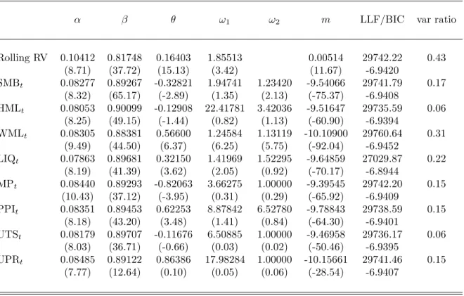
The first row of Table 2 shows the parameter estimates of the GARCH-MIDAS with rolling window RV. Optimal weights ϕj(ω1, ω2) for the GARCH-MIDAS with RV
are monotonically decreasing over the lags so we fixed ω2 = 1 for these models and
left blank at the Table. Note that α + β measures persistence of gδ/t process and
the estimates are 0.9216, which is far lower than the standard GARCH model. This finding is also consistent with Engle, Ghysels, and Sohn (2008) and Engle and Rangel (2008). The resulting conditional market volatility and its long-run component are shown in Figure 1. The dashed line in the first panel represents annualized conditional volatility (p
252τδ/tgδ/t) and the solid line annualized long-run component (
p
252τδ/t).
The τδ/t component in the figure appears to capture very well the long-run persistent
with a nonparametric measure of stock market volatility, we aggregate these components to make them quarterly estimates and show them with quarterly RV in the second panel. When aggregated over a quarter, short-lived shocks gδ/t averages out to one, and we
can confirm this in the second panel of Figure 1; τq·gq and τq share almost the same
dynamics.28 Both of them also fit well with quarterly RV.
For both of our VAR analyses and cross-sectional regressions, we time aggregate our daily volatility components (τδ/t, gδ,t) to monthly components (τt, gt). The summary
statistics of these time aggregated components are shown in Table 1. The autocorrelation structure of τt process shows that τt is quite persistent, but autocorrelations are
substantially reduced by 6th lag and dies out beyond 9th lag. On the other hand, the autocorrelation of gtat the first lag is 0.30 and that is the only significant one. Note
that E[gδ/t] = 1 and the way we time aggregate gδ/t makes the average of monthly gt
very close to the average number of trading days (21 days) in a month for our sample.
4.3
Long-Lag Predictability (GARCH-MIDAS Results)
The GARCH-MIDAS model allows us to directly link wide choice of variables to long-run component τδ/t. All the variables that we are going to consider in this section
are monthly, which means that τδ/t is fixed at given montht. To accommodate a variety
of variables, we adopt equation (12) for modeling τδ/t process instead of equation (9).
Using our GARCH-MIDAS framework, we investigate whether conventional factors such as trading strategy based factors (SMB, HML, WML, LIQ) and macroeconomic factors (MP, PPI, UTS, UPR) contain information about future stock market volatility.
In the context of Section 2, we examine the predictability of stock market volatility. Section 2 adopts a VAR framework to link predictability of stock market volatility and priced factors. If we are able to estimate a VAR model of any order with high precision,
28Sincegδ/t is a unit GARCH(1,1) process, unconditional expectation ofgδ/t is one,i.e. E[gδ/t] = 1.
a VAR approach might be the best way to analyze the relevant predictability relations. However, as we specify the VAR variables in Section 3.2, we have 7 variables for bothy[1]t
and y[2]t and the number of parameters to be estimated will increase in the order of 49 as we increase the VAR order. The predictability relations in a VAR model depend on a choice of variables in the system. On the other hand, the GARCH-MIDAS framework looks at bivariate relations between long-run component τ and a chosen independent variable, and is able to handle a large number of independent variable lags with a small number of parameters. In fact, the number of parameters doesn’t depend on the number of lags used to model the long-run component. However, it comes with the cost of a restrictive structure in coefficients of independent variable lags. Beta function based weighting scheme is quite flexible to accommodate various structures, but it should be pointed out that the sign of all the coefficients to the lags are governed byθand therefore they have all the same signs. These restrictions call for caution when interpreting the impact of the independent variable on the stock market volatility. In a way the MIDAS filter can be looked upon as a low-frequency filter and, in this sense, the predictablity relations revealed by the GARCH-MIDAS might match better with those by VAR with low-frequency data, say quarterly or biannual data. For an empirical implementation, J0 = 36 (months) is chosen, but actual number of lags used in τ modeling will be
determined by the optimal weighting function.
Table 2 shows the results. First of all,θ’s of the GARCH-MIDAS with SMB, WML, LIQ, MP, and PPI turned out to be significant, which implies that these variables do predict the long-run component of stock market volatility. Among these, WML stands out as a best predictor in terms of log-likelihood value (henceforth LLF).29The
GARCH-MIDAS(WMLt) achieves LLF = 29760.64, which is far higher than that achieved by
other models. This can also be verified in Figure 2. It shows that WML captures the
29Note that LLF’s of these models cannot be directly compared with that of GARCH-MIDAS with
long-run component of stock market volatility amazingly well. Among the variables that don’t contain significant information about the future stock market volatility, HML offers the worst fit by LLF = 29735.59. Figure 4 also confirms this. τ(HML) in Figure 4 is flat when compared with τ(W ML) in Figure 2. If a candidate predictor in the MIDAS filter does not contain much information about the future market volatility, the estimation procedure sets θ, ω1, and ω2 such that τ process becomes essentially a
constant and works only as a scale factor to the g process, a unit GARCH(1,1).
To measure how much τ of a certain variable explains the variation of conditional variance estimates (τ ·g), we compute the ratio: V ar(log[τδ/t(•)])/V ar(log[τδ/t(•)gδ/t])
where • refers to a specific variable. We call it a variance ratio and these numbers are also reported in Table 2. It is not suprising to find out that τ(RV) explains 43% of market volatility variation. τ(W ML) andτ(LIQ) also perform quite well with 31% and 22% of variance ratios. The other variables shown to predict market volatility achieve mere 15-16%. Figure 3 also confirms this finding. An interesting observation is that τ(SMB) seems to capture dynamics of long-run component of market volatility pretty well up until 1984, but it decouples from conditional volatility in 1985. Variance ratio also supports the observation: var ratio = 0.2187 (1966-1984) and 0.0495 (1985-1999). Although not reported here, τ(MP) and τ(P P I) show similar behavior. Regrading SMB, this might have something to do with the argument of Hirshleifer (2001) who suggests 1984 as the year in which the disappearance of the size effect first materialized.
4.4
Short-Lag Predictability and Base Factor Estimation (VAR
Results)
Now that we have monthly volatility component series, τt and gt, we can conduct
the VAR analyses discussed in Section 3.2. For a given set of variables in either y[1]t or
y[2]t in Section 3.2, we estimate the VAR model. The order of the VAR was determined
on the basis of the likelihood and the Schwarz’s information criterion (SIC). The optimal order for the VAR with y[1]t is 3 and that with y
[2]
t is 4.
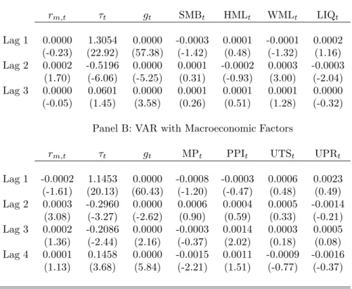
Table 3 and Table 4 show the VAR estimation results. For both of the tables, Panel A shows the VAR results with y[1]t and Panel B with y[2]t . Table 3 shows p-values for the F-tests on each variable. The F-tests reflect the incremental ability of the column variable to predict the respective row variables, given the other variables in the model.30 The asset pricing equation (17) suggests that variables that forecast
either rm,t orτt should be priced. The results in Panel A shows that lags of τ,g, fW M L
strongly predict the long-run market volatility component and the factors generated from these variables are expected have strong explanatory power on cross-sectional variations of mean asset returns. Although not significant at 5% level, fLIQ weakly predicts τ.
Also,fSM B weakly predictsr
m. As was discussed previously, the predictability relations
in a VAR model are affected by the choice of variables in the system. However, the forecasting ability ofτ,g, and fW M L on the long-run stock market volatility component
are robust to various choices of VAR variables and various VAR orders. For some choices of VAR variables and VAR orders,fSM BandfLIQpredictτ quite strongly. However, for
the current specification, fSM B weakly predicts r
m and strongly predicts fW M L which
strongly predicts τ while fSM B does not predict τ directly. The far right column shows
R2 of each equation. R2’s of the equations for fSM B, fHM L, fW M L, and fLIQ are
very low suggesting that the correlations between these and corresponding SM B, HM L,
W M L, and LIQ should be very high; at least 95%.
Panel B of Table 3 shows the VAR F-test results with macroeconomic variables. As in the case with traded factors, τ and g are strong predictors of future τ. In addition to these variables, MP andP P I weakly predicts future stock market volatility.
30In a part, these F-tests investigate which variable predicts stock market volatility. These results
partly answer the main research question that Schwert (1989) answered about two decades ago. However, Schwert (1989) looks at predictability relations between √RV and macroeconomic variables while Table 3 shows the results betweenτt and other variables. Note thatτt·gt is a forecasts of RVt
These predictability relations are also consistent with those revealed by the GARCH-MIDAS model in Table 2. Many have reported that term spread UTS predicts market return and our results also support this finding. We expect MP, PPI, and UTS to be priced across assets. One notable differences in Panel A and Panel B are that R2’s of
equations for the last four variables are higher in Panel B and naturally there are many significant predictors for these variables. Especially, consistent with autocorrelations shown in Table 1, variations of term spread UTS and default premium UPR are explained 92-95%. These results suggest that MP, PPI, UTS, and UPR cannot be deemed as innovations as asserted by Chen, Roll, and Ross (1986). On the contrary, traded factors themselves seem to be good proxies for innovations. Hence, these results support our decision that traded factors themselves are taken as base factors while innovations (•)
of macroeconomic variables are taken as base factors.
One concern with regard to the generated factors from the VAR model is that the VAR system may not, in fact is highly unlikely to contain the full information set used by investors. Also, since the VAR system with yt[1] and one with y
[2]
t contain different
set of variables, τtandgtinnovation factors from these two different VAR systems might
differ much. First of all, the correlation between τt[1]=ftτ[1] from the VAR model with
y[1]t and τt[2]=ftτ[2] from that with y[2]t is 0.90 and correlation between similarly defined ftg[1] and ftg[2] is 0.98; the innovation factors from two different systems are strongly correlated. Secondly, we check if macroeconomic variables in yt[2] should be added to
y[1]t ; we add macroeconomic variables to y
[1]
t one by one to see if the added variable
becomes a significant predictor of any variables in y[1]t . We do the same for the y
[2]
t .
For both robustness checks, in some cases, added variable turns out to be significant in predicting either the added variable itself or market return. However, the increase inR2
of market return equation is marginal. Hence, we conclude that the benefit of adding
y[2] (or y[1]) variables to y[1] (or y[2]) is very limited while innovations to volatility
components from two different VAR specifications are essentially the same.
Table 4 shows parameter estimates forτtequation for both VAR models withyt[1]and
y[2]t . For both specifications, most ofτ andg lags are significant. Note that the variables
(HML, UTS, and UPR) that are not significant in the GARCH-MIDAS results in Table 2 don’t have any significant lags in Table 4, either. For those significant at Table 2, the sign of θ coincide with the sign of coefficient to the significant lag of the corresponding variable in Table 4 except for fLIQ.31 One might think these seemingly consistent
positive/negative relations between stock market volatility and variables of our interest would determine the sign of price of risk of the variable. However, it is not that simple. The asset pricing equation (17) guides us on how prices of risk should be determined. The price of risk of a certain base factor, say ftg[1]=e03
[1]
t , is determined by two part; one that
relates to forecasting future market returns and the other future market volatility. Also, sinceλnandξnare determined as in equation (14)-(15), it is not only the coefficient of one
significant lag, but all the parameters in the VAR model that affect the determination of the price of risk of the factor. Lastly, the structural parameters such as γ and σ should be known beforehand or jointly estimated to determine the price of risk. It is not our interest in this study to recover these structural parameters. Moreover, cross-sectional regressions give us only the price of risk as a whole (i.e. Λn as in equation (18)), but not
a break down of future market return part and future market volatility part. Hence, it is beyond the scope of this paper to examine the theoretical values of prices of risk.
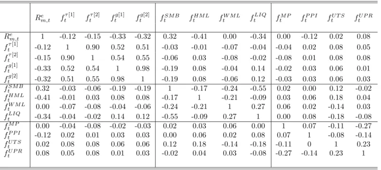
We estimate both VAR specifications and collect the base factors. Table 5 shows the correlation structure of the base factors. It shows the contemporaneous relations among innovations (base factors) to the VAR variables whereas we’ve been so far looking at the time-series relations of VAR variables themselves. Within each group of volatility-based factors, traded factors, and macroeconomic factors, some factors are highly correlated. However, most of factors across the groups show fairly low correlations. Low correlations
31For SMB, there is no significant lag, but the sign of θ in GARCH-MIDAS(SMB) coincides with