IMAGE ANALYSIS DEDICATED TO POLYMER INJECTION MOLDING

IMAGE ANALYSIS DEDICATED TO POLYMER INJECTION MOLDING

DAVID

GARCIA

_GUY

_COURBEBAISSE

_M

_JOURLIN

1_{European Polymer Institute (PEP), 2 rue Pierre et Marie Curie, 01100 Bellignat, France,}2_{ESP, 85 rue Henry} Becquerel, 01100 Bellignat, France,3LISA-ESCPE, 43 Bld du 11 Novembre 1918, 69616 Villeurbanne, France e-mail: [email protected]

(Accepted August 24, 2001)

ABSTRACT

This work follows the general framework of polymer injection moulding simulation whose objectives are the mastering of the injection moulding process. The models of numerical simulation make it possible to predict the propagation of the molten polymer during the filling phase from the positioning of one point of injection or more. The objective of this paper is to propose a particular way to optimize the geometry of mold cavity in accordance with physical laws. A direct correlation is pointed out between geometric parameters issued from skeleton transformation and Hausdorff’s distance and results provided by implementation of a classical model based on the Hele-Shaw equations which are currently used in the main computer codes of polymer injection. Keywords: Hausdorff’s distance, Hele-Shaw equations, injection molding simulation, skeleton.

INTRODUCTION

Injection molding of thermoplastic is a complex process mainly due to the physical properties of the polymers, the processing conditions and the mold geometry. This complexity leads to the development of numerical models, the objectives of which is the simulation of the process. Actually, numerical models integrate the three phases of injection process: the filling phase, the packing phase, and the cooling phase during which the material solidifies. In this paper, we present results dedicated to the optimization of the filling phase. The presented approach consists of finding the optimal location of injection points in order to minimize the pressure required to fill the mold shape. Furthermore, we describe the different steps to achieve this objective. Firstly, we propose a numerical model based on the Hele-Shaw equations to simulate the propagation of the polymer. We use the finite volume method to generate a discrete form of the equations. Secondly, we introduce stereological parameters such as skeleton and Hausdorff’s distance which enable characterization of the geometric properties of the mold shape. Finally, taking in consideration simple shapes, the goal is to show a relevant correlation between the flow simulation given by numerical computation and geometric parameters linked to the mold shape.

PHYSICAL MODEL

Hereafter, we introduce the theoretical background for the presented flow model. We give a brief review of the general equations of fluid dynamics which are the point of departure for flow modelling. Considering

the particular case of injection molding, we use simplifications about material properties and flow characteristics. In fact, the specific shell geometry of molds allows us to consider simplifications commonly called Hele-Shaw assumptions. Furthermore, the computation of polymer propagation necessitates to estimate precisely the position of the polymer/air interface. It allows us to define the boundary conditions of the physical model at each time step.

General equations of fluid dynamics

The fundamental equations of fluid dynamics express the principles of conservation of mass, momentum and energy. The three fundamental equations of conservation in their local form are the following (Candel, 1995):

– Equation of mass conservation,

dρ

dt ρ∇v 0 (1)

– Equation of momentum conservation,

ρdv

dt ∇p ∇σ

n ρg (2)

– Equation of conservation of energy,

ρ d dt e 1 2v 2

∇q ∇σv ∇pv ρg v

(3)

with ρ the density, v the velocity, p the pressure, σ

n

the inertial and gravitational terms will not be taken into account in the momentum equation. This simplification leads to a well known equation: the

∇v 0 (4)

∇p ∇ σ

n 0 (5)

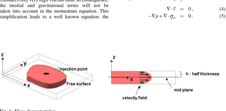
Fig. 1. Flow characteristics.

Hele-Shaw assumptions

During the filling phase, the flow into the mold cavity is very similar to a laminar flow between two plates with a very thin gap (Fig. 1).

We consider a cartesian coordinate system, as shown in the Fig. 1 (where the z-axis is in the thickness direction and the x-y plane is on the mid plane of the cavity) and the velocity components u,v and w are respectively taken in the x, y and z directions. The Hele-Shaw flow model consists of the following assumptions (Kennedy, 1995):

– The w component of the velocity is neglected with respect to the others components.

– The pressure constant in thickness, is a function of x and y.

– The velocity gradient in the x and y directions is negligible with respect to z direction.

Applying the Hele-Shaw assumptions to the Stokes’s equation, we obtain the simplified equations:

∂p

∂x

∂ ∂z

η∂_∂u

z (6) ∂p ∂y ∂ ∂z

η∂v ∂z

(7)

∂p

∂z 0 (8)

withη the viscosity. By integrating the mass and the momentum equations with respect to the thickness direction, we obtain a single equation for pressure which combines mass conservation and momentum conservation. The final result gives the following Laplace’s equation (Kennedy, 1995).

∂ ∂x

S∂p

∂x

∂

∂y

S∂p

∂y 0 (9) with: S h 0 z2

ηdz (10)

Eq. (8) means that, at each time step, the pressure field is the solution of equation (9) with a zero pressure Dirichlet boundary condition applied at the free-surface.

DISCRETE MODEL

(a) (b)

Fig. 2. (a) Control volume and flux. (b) Illustration of free surface cells.

The finite volume method (Eymard et al., 1997) allows us to provide an accurate numerical scheme for the resolution of the pressure Eq. (9) which drives the flow during the propagation. The volume of fluid method uses a scalar quantity C, called cell’s concentration defining the position of the fluid in the domain. The value C is equal to 1 if the cell is completely occupied by the fluid and 0 if empty. The free surface location is given by the set of empty or partially full cells which are neighbour to full cells. These cells are called free surface cells (Fig. 2b). Considering the position of the fluid at time t, we solve the pressure equation by applying Dirichlet boundary

conditions on free surface cells and a constant flow rate at the injection point location. Dirichlet boundary conditions correspond to a zero value for pressure on free surface cells. The concentrations are updated in accordance with the volume of fluid method (Hirt

et al., 1981). The new concentration values define

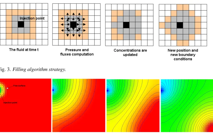
the new position of the fluid and new boundary conditions for the pressure equation. The movement of the fluid is performed by successive iterations. An illustration of one iteration is provided in Fig. 3. A result of computation is shown (Fig. 4) for an isotherm newtonian viscosity’s law.

Fig. 3. Filling algorithm strategy.

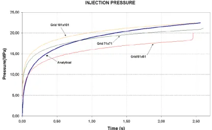
Fig. 5. Injection pressure Pi_analytical and Pi_numerical.

VALIDATION ACCORDING TO A REFERENCE MODEL

In order to estimate the accuracy of the numerical model, we choose to compare it with a well known analytical model: the disk mold. The principle consists of studying the radial flow between two parallel plates from a central injection point. The equation of injection pressure P_i and the front position are expressed as (Agassant et al., 1989):

R_analyticalt

Qt

2πh R

2

0 (11)

Pi_analytical

3ηQ

4πh3ln

R R₀

(12)

where Q is the flow rate, h the half thickness between the plates, t the time,η the viscosity and R₀the initial front radius. The assumptions are those of Hele-Shaw for an isotherm newtonian fluid. Firstly a comparison between the numerical front propagation radius for different resolutions and the radius curve provided by the analytical model gives a high correlation. Secondly in the same way, we show the difference between the analytical injection pressure and numerical results (Fig. 5). It is due to the spatial resolution. To avoid this difference a mesh refinement must be performed.

SKELETON AND HAUSDORFF’S DISTANCE

In this section, we introduce a mathematical morphology transformation (Serra, 1988) and a metric in order to characterize mold shapes. The considered transformation is the well known skeleton. The skeleton of the set A is defined by the family of centers

of all maximal disks defined in A (Fig. 6c to Fig. 9c). A maximal disk Dx r is one which is included in the

set A, but not strictly included in any other disk in A. The considered metric is the Hausdorff’s distance (Rucklidge, 1995) allowing to measure the distance between two sets of points. Given two sets A and B, the definition of the Hausdorff’s distance is defined as:

HA B maxhA B hB A (13)

hA B max

a A

min

b B

da b (14)

hB A max

b B

min

a A

da b (15)

where da b is the Euclidean distance. The function

hA B is called the directed Hausdorff’s distance from

A to B. Taking into account a mold and its injection

point, the set A is the boundary of the mold and the set B is the injection point. The distance map (Fig. 6b to Fig. 9b) is the result of Hausdorff’s distance computation when injection point takes successively all the possible position inside the shape. Each level set corresponds to the set of injection point locations which leads to the same Hausdorff’s distance value. In the case of Figs. 8b and 9b the computation is matched in the sense that we cannot use the Euclidean distance but the geodesic distance.

NUMERICAL RESULTS

(a) (b) (c)

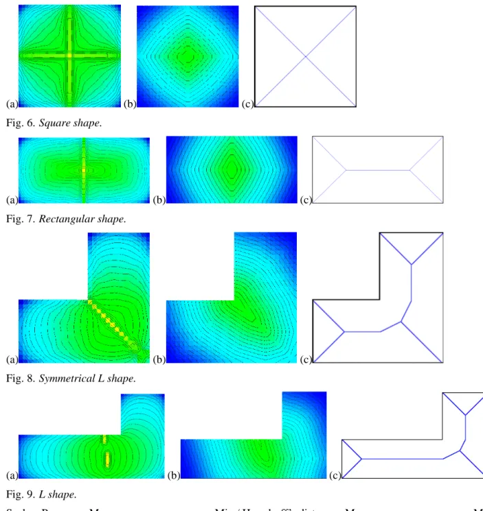
Fig. 6. Square shape.

(a) (b) (c)

Fig. 7. Rectangular shape.

(a) (b) (c)

Fig. 8. Symmetrical L shape.

(a) (b) (c)

Fig. 9. L shape.

Scales: Pressure - Max Min / Hausdorff’s distance - Max Min

The numerical results are performed for different shapes: square shape (Fig. 6), rectangular shape (Fig. 7), symmetrical L shape (Fig. 8) and a L shape (Fig. 9).

INTERPRETATION OF RESULTS

AND CONCLUSION

In the case of Figs. 6 and 7, we observe a direct spatial correlation between geometric parameters and the locus of minimum injection pressures. Concerning geometric parameters, we associate the minimum of the Hausdorff’s distance to the center of the maximal

forme des mati`eres plastiques. Paris: Lavoisier. Candel S (1995). M´ecanique des fluides, 2nd Ed. Paris:

Dunod.

Eymard R, Gallou T, Herbin R (1997). Finite Volume methods. Prepublication.

Garcia D, Courbebaisse G, Jourlin M (2000). An investigation of mathematical imaging toward simulation of polymer injection molding. Proc 16th IMACS 2000 World Congress.

Hirt CW, Nichols BD (1981). Volume of fluid (VOF)

Molding Simulation: A Mathematical Imaging Approach Based on Propagation of Discrete Distances. Comp Mater Sci 18(1):19-23.

Kennedy P (1995). Flow analysis of injection molds. M¨unchen: Hanser.

Ruckildge W (1995). Efficient visual recognition using the Hausdorff’s distance. Lecture Notes on Computer Science no. 1173. New York: Springer Verlag.