ON ESTIMATION AND HYPOTHESIS TESTING OF THE GRAIN SIZE
DISTRIBUTION BY THE SALTYKOV METHOD
Y
URIG
ULBINDepartment of Mineralogy, Crystallography and Petrography, Saint-Petersburg Mining Institute, 2, 21 line, 199106 Saint-Petersburg, Russia
e-mail: [email protected]
(Accepted October 22, 2008)
ABSTRACT
The paper considers the problem of validity of unfolding the grain size distribution with the back-substitution method. Due to the ill-conditioned nature of unfolding matrices, it is necessary to evaluate the accuracy and precision of parameter estimation and to verify the possibility of expected grain size distribution testing on the basis of intersection size histogram data. In order to review these questions, the computer modeling was used to compare size distributions obtained stereologically with those possessed by three-dimensional model aggregates of grains with a specified shape and random size. Results of simulations are reported and ways of improving the conventional stereological techniques are suggested. It is shown that new improvements in estimating and testing procedures enable grain size distributions to be unfolded more efficiently.
Keywords: computer simulation, grain size distribution, planar section, Saltykov method, stereology.
INTRODUCTION
The grain size distribution is of considerable importance in understanding the microstructure of rocks, ceramics, alloys and so on. In studying opaque mediums it is convenient for scientists to observe grain aggregates in thin or polished sections. Stereological techniques are used for converting two-dimensional grain size measurements into three-dimensional data. In the case that an aggregate consists of second-phase grains and the surrounding matrix second-phase, a conventional solution of the unfolding problem introduced by Wicksell (1925) is the back-substitution method advanced by Scheil (1931; 1935) and Schwartz (1934) and later modified by Saltykov (1970). The original method has been proposed for estimating the size distribution of embedded grains assuming that they are spherical in shape and their centers are randomly dispersed within the specimen. With these assumptions,a planar sectionof an aggregate is made and the histogram of diameters of grain sections, based on size classes of equal width∆=Rmax/q, where Rmax
denotes the maximum diameter of intersections in the sample, q is the number of size classes, is obtained. Classes are numbered, the first being the smallest, and diameters of all grain sections relating to class i are assigned a value of its upper bound,
Ri=∆i, i=1,2, . . .q.
In a similar manner, diameters of all grains falling in class j are given by
rj=∆j, j=1,2, . . .q.
From geometrical considerations it follows that grain sections of class i come from the grains of each class j (j>i), which centers are placed at a distance
(∆/2)pj2−i2 <l ≤ (∆/2)p
j2−(i−1)2 from the
planar section. Consequently, the intensity of grain sections nRi (the number of grain sections in class i per unit area of the intersected plane) may be derived from the linear equation system
nRi =∆
q
∑
j=1Bi jnrj, i=1,2, . . .q, (1)
where nrj denotes the unknown intensity of grains (the number of grains in class j per unit volume of the specimen), coefficients Bi jare (Saltykov, 1970):
Bi j=
p
j2−(i−1)2−pj2−i2,
0,
i≤ j, i> j.
The required nrj is found from (1) by back-substitution for nRi:
nrq= 1
∆
nRq Bqq
,
nrq−1= 1
∆
1
Bq−1,q−1
nRq−1− Bq−1,q Bq−1,q−1Bqq
nRq
,
nrq−2= 1
∆
1
Bq−2,q−2
nRq−2− Bq−2,q−1 Bq−2,q−2Bq−1,q−1
nRq−1
−
Bq−2,q
Bq−2,q−2Bqq −
Bq−2,q−1Bq−1,q
Bq−2,q−2Bq−1,q−1Bqq
nRq
,
The solution can be written in the form (Saltykov,1970, p. 283; Stoyan et al.,1987)
nrj= 1
∆ q
∑
i=jAi jnRi , j=1,2, . . .q, (2)
where Ai j denotes transition coefficients that are depended on q and cited for example by Russ and DeHoff (2000). They can be generalized as follows:
Ai j=
Tii, i= j,
− j−1
∑ m=i
AmiTm j, i< j.
where Ti j denotes coefficients defined by (Takahashi and Suito, 2003):
Ti j=
1
Bj j
, i= j, Bi j
Bj j
, i< j.
To improve stereological techniques, S. A. Saltykov simplified the calculation procedure described above and extended this unfolding method to arbitrary convex grains. For adapting the theoretical model to the practical needs, he substituted the discrete analogue for the basic stereological equation, having introduced the geometric scale of size classes instead the linear one at the same time (Saltykov, 1970, pp. 302-311). Let N(r), N(R) be the distribution function of the size of grains r and that of grain sections R respectively. Furthermore, let NV, NA be mean numbers of grains per unit volume and grain sections per unit area respectively. The general formula relating named quantities together is
NAN(R) =bNV Z ∞
R
r·p(r,R)dN(r), (3)
where p(r,R) denotes a conditional distribution function of R, given that r has taken a particular value, b is a shape factor. For spherical grains Eq. 3 rearranges to
NA[1−N(R)] =NV Z ∞
R
p
r2−R2dN(r), (4)
(cf. Ohser and Nippe, 1997; Ohser and Sandau, 2000). Considering Eq. 3 and starting from the two-dimensional data histogram based on size classes that form a geometric series
Ri=Rmaxaq−i, i=1,2, . . .q,
0<a<1, one can derive follow discrete expressions:
nRi =NA[N(Ri)−N(Ri−1)] ,
pi j=p(rj,Ri)−p(rj,Ri−1),
pi j=pq+i−j.
The last expression presented here points up the fact that the probability pi j in the case of geometric discretization depends on the difference of indices
(i−j) only. In view of derived formulae, Eq. 3 can be transformed into the system of linear equations
nRq=nrqpq¯rq
nRq−1=nrq−1pq¯rq−1+nrqpq−1¯rq
nRq−2=nrq−2pq¯rq−2+nqr−1pq−1¯rq−1+nrqpq−2¯rq
. . .
which is represented in a concise form
nRi =
q
∑
j=inrjpq+i−j¯rj, i=q,q−1, . . .1, (5)
where ¯rj denotes the mean caliper diameter of grains in class j (corresponding to the upper limit of the size interval), pq+i−j is the probability that such a diameter of a random intersection of a body whose shape approximates the shape of grains will fall into a particular size class. It should be remarked that the concept of a mean caliper diameter (i.e., a distance between two parallel planes that are tangent to a grain measured in any direction) is used here in the context of the governing stereological relationship
NA=¯r·NV , (6)
which holds for non-sphericall convex grains (Russ and DeHoff, 2000).
The solution of Eq. 5 is given by
nrq= n
R q
pq¯rj
nrq−1=n
R
q−1−nrqpq−1¯rq
pq¯rj
nrq−2=n
R
q−2−nrq−1pq−1¯rq−1−nrqpq−2¯rq
pq¯rj
. . .
or
nrj= 1
pq¯rj
nRj − q−1
∑
i=jnri+1pq+j−i−1¯ri+1
! ,
j=q,q−1, . . .1,
(7)
of transition coefficients Cq+j−i can be obtained and simplified version of Eq. 7 can be given by (Ohser and Nippe, 1997):
nrj=
q
∑
i=jCq+j−inRi, j=q,q−1, . . .1. (8)
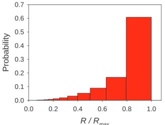
As in the previous case, this formula is obtained assuming that the maximum size of grain sections is the maximum size of grains in the sample. It is spherical grains that fulfill the last condition best of all thanks to the shape of the intersection diameter distribution for a sphere (Fig. 1). Since the largest section circle is probably associated with the largest sphere in the sample, one can subtract the corresponding number of intersections from the numbers of ones of each smaller class iterating the process for the size classes that follow the largest one until all of them are accounted for.
R / Rmax
0.0 0.2 0.4 0.6 0.8 1.0
Probability
0.0 0.1 0.2 0.3 0.4 0.5 0.6 0.7
Fig. 1. Probabilities of random intersections for a
sphere.
The probability pi of finding a specified shape body section in corresponding size class is required to implement Eq. 7 for unfolding. In the case of sphere this probability can be computed by the well-known analytical expression
p(Ri−1<R<Ri) =
q
1−R2i−1−
q
1−R2i ,
where Ri−1 and Ri denote a lower and upper bound
of a given size class respectively. Similar expressions for non-spherical bodies are also available. Mainly this is true for spheroids (Cruz-Orive, 1978); as for polyhedra, the only probability that an intersection of some polyhedron (e.g., prism or tetrahedron) has a given number of vertices was derived (Sukiasian, 1982; Voss, 1982), whereas the analytical expression
for pi remains to be obtained (Ohser and Sandau, 2000). Only recently has it been possible to evaluate some probabilities of interest with numerical routines and to apply stereological techniques for unfolding the size distribution of non-spherical grains (Ohser and Nippe, 1997; Han and Kim, 1998; Sahagian and Proussevitch, 1998; Higgins, 2000; Ohser and M¨ucklich, 2000).
In spite of apparent progress (and in many respects owing to it), the validity of the stereological conversion has been the focus of considerable recent attention. Both theoretical and empirical approaches to the problem have been applied. The former appeals to the concept of the condition number as a measure of stability and error sensitivity during the numerical analysis of linear systems (Kanatani and Ishikawa, 1985). It has been demonstrated that condition numbers of matrices of stereological coefficients in linear systems of the type (1) or (5) are rather small in order to consider numerical solutions being discussed as computationally stable (Ohser and Sandau, 2000). The algebraic treatment has been complemented by experimental studies of the stereological estimation error. With full-scale and model tests, grain size distributions unfolded by the Saltykov method or alternative stereological procedures were compared with actual ones, which arise from additional investigations of specimens via independent techniques (Karasev and Suito, 1999; Susan, 2005) or derive from computer simulations (Bl¨odner et al., 1984; Takahashi and Suito, 2001; Xu and Pitot, 2003). Assuming spherical shape of grains, experimental evidence points to the fact that although the intensity nrj can be predicted reasonably well with unfolding, the total number of grains per unit volume NV is often underestimated against the true value (Takahashi and Suito, 2003). As this takes place, the mean grain diameter m is overestimated due to the omission of small grain sections (Susan, 2005). Unfolding data are slightly effected by the number of size classes (provided it lies between 15 and 25) but highly susceptible to the number of observed grain sections (which is advised should be range from several hundred to several thousand). While the Saltykov method offers some advantages over alternative stereological procedures, it along with them is unable to verify hypothesized diameter distribution with goodness-of-fit tests owing to computational errors (Bl¨odner et al., 1984).
of parameter estimation and to justify the possibility of testing statistical hypotheses about the functional form of an expected grain size distribution for the stereological conversion. In an effort to handle these issues, the computer modeling was used to match size distributions obtained stereologically with those possessed by three-dimensional aggregates of grains with a same shape and random size. A sphere and rhombic prism were chosen as assumed model shapes since they are often employed to approximate a habit of crystal inclusions in natural and artificial matters. For instance, the spherical shape can be used to approximate the rhombic dodecahedron crystals of garnet in metamorphic rocks as well as the prismatic shape is suitable for approximation of tabular crystals of plagioclase in basalts. In view of the fact that the shape can vary along with the size of grains, there are several works, which attack the problem of stereological estimation as applied to the bivariate size-shape distribution (Wicksell, 1926; Cruz-Orive, 1976; 1978; Møller, 1988; Bene˘s et al., 1997; Ohser and M¨ucklich, 2000). However, in studies of specimens like rocks, where the shape of grains is typically invariable due to similar conditions of crystallization, the topical problem is to unfold the solely the grain size distribution. With this in mind, to improve results of unfolding with reference to prismatic grains, the Saltykov method was developed having regard to intersection histogram properties for a prism with a given aspect ratio. The manner of verification of the expected diameter distribution with the minimum chi-square method of parameter estimation was advanced. On this basis, the evaluation of statistics for stereological estimators was made as a function of the amount of sampling.
STEREOLOGY OF SPHERES
It was the stereology of spherical grains that the first series of simulations dealt with. In each simulation, the test volume was filled with the large number of randomly located spheres with random diameters. After that, cutting the volume by a set of parallel planes, which are apart from each other at a distance exceeding the diameter of the largest sphere in the population, the intersection diameter histogram was constructed from the geometric discretization with a = 10−0.1, q = 20. In so doing, overlapping intersections, whose contribution was negligible due to large spaces between centers of spheres as compared with their diameters, were considered together with non-overlapping ones. On the basis of two-dimensional data, the intensity of spheres was estimated fromEq. 7, where ¯rjas used here denotes the
diameter of section circles lying in class j, pq+j−i−1is
the analytical probability for the diameter of a random intersection of a unit sphere to fall in corresponding size class.
For verifying a hypothesized diameter distribution from unfolded data it is advisable to use the chi-square (χ2) goodness-of-fit test (Cram´er, 1946). It may be
carried out only on independent observations, which are put into categories, not on relative frequencies, average values, or other derived data. Hence, this test is not applied to compare the unfolded diameter distribution and that of spheres forming the model aggregate,as was done by Bl¨odner et al. (1984). On the other hand, as discussed byNadelhaft (1973)and Han and Kim (1998), this test is applied to compare the observed diameter distribution and that of intersection of spheres, which would form the aggregate in the case their diameter distribution is identical to the unfolded one.
To construct the intersection diameter distribution refers to the unfolded one, estimation of parameters of the sphere diameter distribution was made from unfolded data by the maximum likelihood method. The main problem, which arises in this context, is a frequent appearance of negative intensities of sphere sections in small classes due to errors caused by inaccuracy in the determination of intensities of sphere sections in large ones and accumulated during the successive subtraction by Eq. 7. Taking into account that negative intensities are slight, one can neglect them without appreciable loss of accuracy, especially, as will be shown below, they play no part in definitive estimation of parameters.
The next step was a calculation of the expected intensity of spheres nrj∗ from estimated parameters, whereupon the expected intensity of sphere sections
nRi∗was derived from the following equation
nRi∗=
q
∑
j=inrj∗pq+i−jrj, i=1,2, . . .q, (9)
which is equivalent to Eq. 5. When corrected for a sum of observed intensities, the expected intensities of sphere sections (i.e., theoretical probabilities for the test model) coupled with the observed ones were used to calculate the chi-square test statistics
D=
l
∑
i=1
nRi −
q ∑ i=1
nRi n
R∗ i q ∑ i=1
nR∗
i
2
q ∑ i=1
nR i
nR∗
i q ∑ i=1
nR∗
i
As part of a calculation, adjacent expected intensities were combined if one of them was less then 5 (Sheskin, 2000).
It is known that the limiting distribution of the chi-square statistic in the case of a composite null hypothesis depends on which method is applied for estimation of the parameters of a hypothesized distribution. In this connection it would appear natural to look for the ‘best’ values of unknown parameters capable of making the value of D as small as possible. Under reasonably general conditions, minimum chi-square estimation outlined above coincides with the maximum likelihood method for grouped data. In both cases, under the assumption that a null hypothesis is true, the chi-square statistic is asymptotically (as the sample size tends to infinity) distributed as a χ2 random variable with(w−u−1)degrees of freedom, where w denotes the number of bins, u is the number of parameters in the hypothesized distribution to be estimated (Cram´er, 1946). Note that the estimator based on the sample vector from the multinomial distribution cannot be replaced here by the maximum likelihood estimator for ungrouped data (Chernoff and Lehmann, 1954). Generally, the calculation of such an estimator is only possible numerically, as is the minimum chi-square estimator. Some examples of numerical routines for the minimum chi-square method were reported (Ratcliff and Tuerlinckx, 2002).
On this basis, minimum chi-square estimation by adjusting parameter values of the unfolded distribution was chosen to obtain the proper distribution of D. With this aim in mind, a value of each unknown parameter was searched in the vicinity of its initial estimate. The routine of searching consisted of an enumeration of series of values in intervals which covered initial estimates and had widths equal to 20% of them. Among these values, the ones that yielded a minimum for the chi-square statistic were selected. The minimized value of D was used to test the hypothesis H0 that the observed intensities of
sphere sections correspond to the expected ones. If this hypothesis was accepted, it is inferred that there is no significant discrepancy between the unfolded intensities of spheres and the actual ones.
During the modeling procedure several types of sphere diameter distributions (lognormal, gamma, Rayleigh, Weibull, etc.) were simulated. As an example, the conditions used in one of the simulation sets provided for spheres whose diameters are lognormally distributed, are given in Table 1.
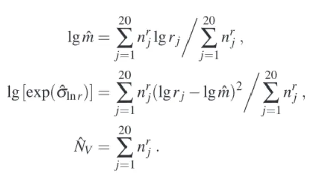
The results obtained appear in Fig. 2 and Table 2. The parameter estimators are herein calculated from
formulae
lg ˆm=
20
∑
j=1nrjlg rj
20
∑
j=1nrj,
lg[exp(σˆln r)] = 20
∑
j=1nrj(lg rj−lg ˆm)2 20
∑
j=1nrj,
ˆ
NV =
20
∑
j=1nrj.
The histogram based on twenty size classes was used to evaluate estimators of m and σln r. Their
relative standard errors are no more than 2–5% with the estimators only slightly biased toward large size classes at the same time. Negative and positive deviations from true parameter values, which observed in a single simulation, are less than 4–5 and 9–10%, respectively. Both accuracy and precision of estimation usually increased provided they are evaluated by minimization of the statistic D.
The value of the estimator of NV was obtained from the summation of unfolded intensities of spheres. In the course of the summation, the negative intensities
nri were omitted, because otherwise underestimation of NV prevails. Furthermore, it has appeared useful to increase the number of size classes (e.g., from 20 to 80) for extracting an virtually unbiased estimator of that parameter. As a consequence, its relative standard error and bias are 4 and 1%, respectively.
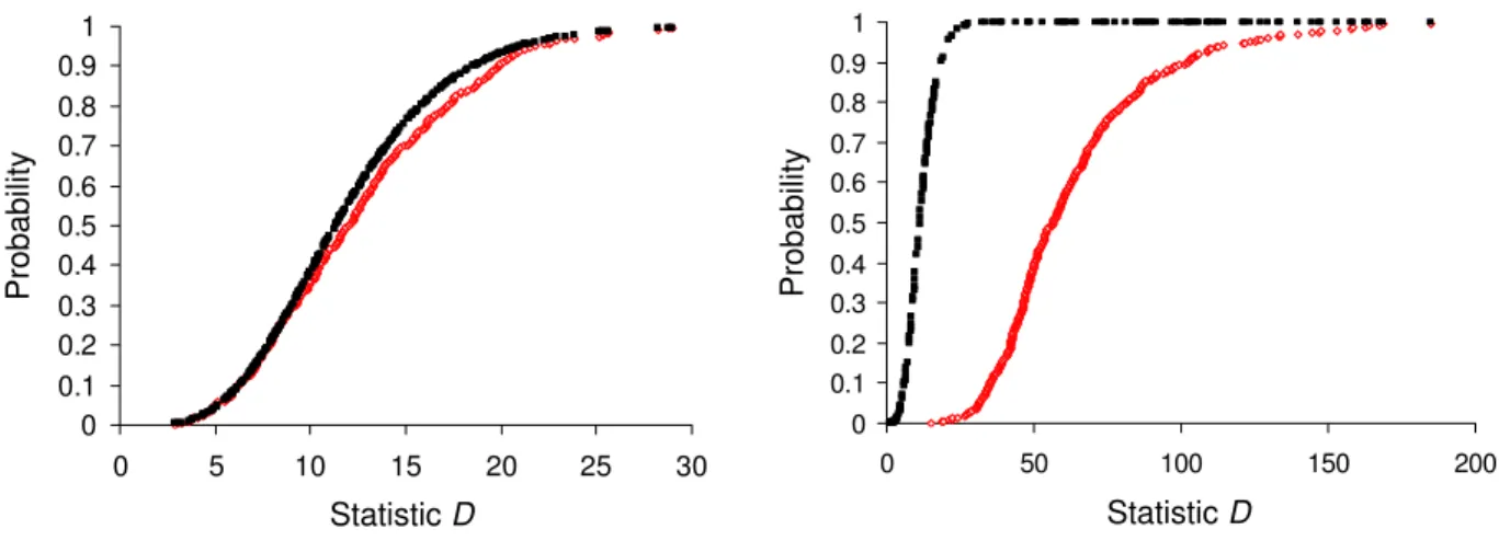
The experimental distribution function of minimized D, which is calculated when the null hypothesis H0 is true, follows nearly the theoretical
χ2
w−3 distribution fuction. When the alternative
hypothesis H is true, which is close to the null hypothesis (for instance, if the observed section diameter distribution is associated with spheres whose diameters are Rayleigh distributed), the power of the test is found to be near one (Fig. 3).
Table 1. Conditions for the sphere diameter distribution simulation set.
Number of simulations 300
Number of spheres per test volume, NV 30000 Number of sphere sections per area of
test planes, NA
2000
Number of size classes of diameter histograms, q
20
-1000 0 1000 2000 3000 4000 5000 6000
0.00 0.01 0.02 0.03 0.04 0.05 0.06
Diameter of spheres
In
te
n
s
ity
o
f
s
p
h
e
re
s
0 50 100 150 200 250 300 350 400 450
0.00 0.01 0.02 0.03 0.04 0.05 0.06
Diameter of sphere sections
In
te
n
s
ity
o
f
s
p
h
e
re
s
e
c
tio
n
s
Fig. 2. Left: actual sphere diameter distribution (solid line) and unfolded one (dotted line). Right: observed
section diameter distribution (dotted line) and expected one (solid line). D=5.53,χ02.05;12=21.03.
0 0.1 0.2 0.3 0.4 0.5 0.6 0.7 0.8 0.9 1
0 50 100 150 200
Statistic D
P
ro
b
a
b
ili
ty
0 0.1 0.2 0.3 0.4 0.5 0.6 0.7 0.8 0.9 1
0 5 10 15 20 25 30
StatisticD
P
ro
b
a
b
ili
ty
Fig. 3. Probability distribution functions of the statistic D for spheres (red) andχ122 distribution (black) if the null hypothesis H0is true (left) or the alternative hypothesis H is true (right).
Simulation results for alternative types of sphere diameter distributions are closely similar to one another. In particular, for the Rayleigh distribution, the relative standard error and bias of the estimator of the scale parameter are each no more than a few percent as before. The same is true for the estimator of NV. Also, the empirical distribution function of D, found under the null composite hypothesis, follows the theoretical chi-square distribution function, if not as near. The small gap between the empirical and theoretical distribution here is probably explained by dependence of the limiting distribution of D from a manner of binning(Lemeshko et al., 2007). Whereas one can use logarithmic data and an arithmetic series of histogram classes for the lognormal distribution, it is forced to apply raw data and a geometric series of histogram classes for the Rayleigh distribution. Even with a combination of classes in the tails of
a histogram, the both modes of binning are non-optimal to test a distribution (although possibly the uniform binning in a less degree than the non-uniform one). Because the limiting distribution of D lies between χw2−1 and χw2−u−1 distributions in this situation (Lemeshko et al., 2007), the probability that the chi-square test statistic does not exceed a given value is found to be understated when using the χ2
Table 2. Results of parameter estimation for the sphere diameter distribution simulation set. Hereafter, values
in parentheses are maximum likelihood statistics of parameter estimators, values in front of parentheses are statistics computed by minimization of D.
Estimator Mean Standard error Relative standard error, % Relative bias, %
ˆ
m 0.0102 (0.0103) 0.0002 (0.0003) 2 (3) 2 (3)
ˆ
σln r 0.512 (0.503) 0.0108 (0.0254) 2 (5) 2 (1)
ˆ
NV 30409 1114 4 1
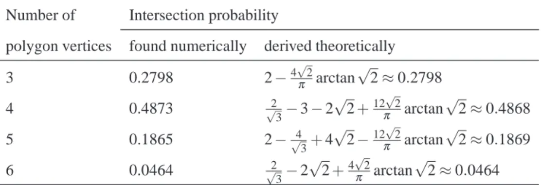
Table 3. Probabilities that random intersections of a cube have a given number of vertices
Number of Intersection probability
polygon vertices found numerically derived theoretically
3 0.2798 2−4√π2arctan√2≈0.2798
4 0.4873 √2
3−3−2
√
2+12π√2arctan√2≈0.4868
5 0.1865 2−√4
3+4
√
2−12π√2arctan√2≈0.1869
6 0.0464 √2
3−2
√ 2+4√2
π arctan
√
2≈0.0464
STEREOLOGY OF PRISMS
The stereology of prismatic grains was the objective of the next series of simulations. In each simulation, the test volume was filled with the number of randomly oriented rhombic prisms (rectangular parallelepipeds) that had a random size and a fixed aspect ratio of a : b : c, a<b<c. It is axiomatic that
centers of prisms were distributed in a Poisson field with a constant density which was sufficiently low to neglect overlapping effects. To ensure the randomness of a specified direction of a prism ~E(ϕ,θ), where ϕ, 0≤ϕ <2π denotes longitude (the angle between the positive X axis and the orthogonal projection of the direction on the XY plane),θ,−π/2≤θ ≤π/2 is latitude (the angle between the direction and its orthogonal projection on the same plane), a random value uniformly distributed in [0,2π) for ϕ and that in [−1,1] for sinθ were taken (cf. Cruz-Orive, 1997). The final position of a prism was attained by rotating around that direction with the random angleψ, 0≤ψ<2π uniformly distributed in[0,2π). Matrix operations were used to perform translations and rotations necessary for simulations (see, e.g., Han and Kim, 1998; Ohser and M¨ucklich, 2000).
After cutting the volume by a set of planar sections, the length of the longest side R1, the length
R2 (the longest dimension) and the breadth R3 (the
size measured in the direction normal to the longest
side) of section polygons were measured (Fig. 4). One of three kinds of measured sizes, namely, the length R1 was used to generate the intersection size
histogram. In choosing between the sizes, a preference has been given to those conveniently measured by hand. The histogram was arranged from the geometric discretization without considering overlapping effects over again.
Fig. 4. Measurements of the longest side (solid lines),
the length (dashed lines) and the breadth (dotted lines) of prism polygon sections.
Much the same procedure works efficiently for calculation of sets of probabilities pi for prisms with
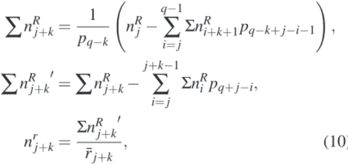
Following equations were developed to unfold the prism size distribution from measurement data
∑
nRj+k= 1pq−k
nRj −
q−1
∑
i=jΣnRi+k+1pq−k+j−i−1
! ,
∑
nRj+k′=∑
nRj+k−j+k−1
∑
i=jΣnRi pq+j−i,
nrj+k=Σn
R j+k′ ¯rj+k
, (10)
j=q,q−1, . . . ,1. Formulae were derived allowing for the fact that the modal size class (q−k) of prism
sections is generally not the largest size class q as illustrated in Fig. 5. Therefore, the maximum size of prism sections is very likely not the maximum size of prisms in the sample, particularly when the number of intersections available for observation is limited. Neglect of this may introduce large errors into unfolding data (Sahagian and Proussevitch, 1998; Higgins, 2000).
Fig. 5. Probabilities of random intersections for a
prism with aspect ratio 1 : 1 : 5.
In the first stage of the calculation, the total number of intersections ΣnRj+k associated with the prisms of size class ( j+k) wasapproximatedtaking into account the contributions from intensities of prisms of lager classes,
ΣnRq+k= 1 pq−k
nRq ,
ΣnRq+k−1= 1 pq−k
nRq−1−ΣnqR+kpq−k−1
,
ΣnRq+k−2= 1 pq−k
nRq−2−ΣnRq+k−1pq−k−1
−ΣnRq+kpq−k−2
, . . .
Thereafter, the the resulting value was adjusted considering the contributions from intensities of prisms of smaller classes,
ΣnRq+k′=ΣnRq+k−ΣnRqpq−ΣnRq+1pq−1
−ΣnRq+2pq−2−. . .−ΣnRq+k−1pq−k+1,
ΣnRq+k−1′=ΣnRq+k−1−ΣnRq−1pq−ΣnRqpq−1
−ΣnRq+1pq−2−. . .−ΣnRq+k−2pq−k+1,
ΣnRq+k−2′=ΣnRq+k−2−ΣnRq−2pq−ΣnRq−1pq−1
−ΣnRqpq−2−. . .−ΣnRq+k−3pq−k+1,
. . .
The refined total number of intersections ΣnRj+k′
was used to calculate the required intensity nrj+k,
nrq+k=Σn
R q+k
′
¯rq+k
,
nrq+k−1=Σn
R q+k−1
′
¯rq+k−1
,
nrq+k−2=Σn
R q+k−2′
¯rq+k−2
,
. . .
When calculating nrj+k values, the mean caliper diameter of prisms in class j+k should be obtained.
Note in this connection that for the chosen mode of normalization of data, the upper bound of the largest size class of the prism section histogram (similar those shown in Fig. 5) corresponds to the largest diagonal of the prism face bc (subject to the longest side of a prism section is measured as the size of an intersection). It follows that the long edge of prisms in class j+k can
be given by
cj+k=
rj+k √
b2+c2 .
Considering that
¯rj+k=
a+b+c
2 cj+k, (cf.Russ and DeHoff, 2000), this yields
¯rj+k=rj+k
a+b+c
2√b2+c2 .
given classwas changed once again by the long edge of a prism in that class from
cj+k=¯rj+k 2
a+b+c,
to provide unbiased estimators of interest.
A common undesirable effect resulting from the calculation by Eq. 10 is an appearance of negative intensities of prism sections not only in the left, but also in the right tail of the unfolded distribution. As noted above for spheres, these intensities are rather weak and could be ignored in estimating of some parameters of the distribution (like mean and standard deviation),especially since initial estimates adjust byminimization of the chi-square test statistic. Nevertheless, for prisms as opposed to spheres, these intensities must not be ruled out in estimating of the number of spheres per test volume. Experiments show that every so often the value of ˆNV computed by the summation of unfolded intensities without considering negative ones is overestimated. Thus one should taking into account positive intensities as well as negative ones to obtain the value of the estimator that is closer to the true value.
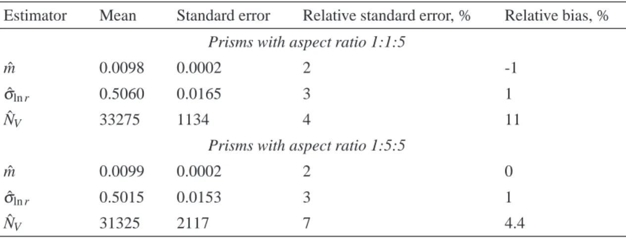
Several types of prism size distributions, including the lognormal, were simulated as part of the unfolding procedure. When this takes place, the shape of prisms changed from columnar (with the aspect ratio 1 : 1 : 5) to tabular (with the aspect ratio 1 : 5 : 5). To verify unfolding data, the original hypothesis on similarity between unfolded and actual prism size distributions was invariably replaced by the hypothesis on similarity between observed and expected intersection size ones. The results of a selection of the simulations, made under conditions similar to those described previously in Table 1, are shown in Fig. 6 and Table 4. They are not too different from those obtained for spheres. Such is the case both with parameter estimation and the distribution of the minimized chi-square test statistic referring to Fig. 7.
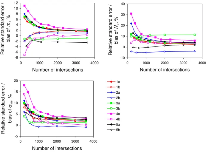
For spheres and prisms alike, the accuracy and precision of estimation is a function of the amount of sampling, as demonstrated by the dependence between statistics of estimators and the number of intersections (Fig. 8). One and half thousand or two thousand sections are generally enough to obtain estimators with the standard error not exceeding 2–3% (when estimating the local and shape parameter of the size distribution) else 4–7% (when estimating the number of grains per test volume). Here, relative errors encountered in a single simulation comprise roughly no more than 10–20%, increasing from columnar to tabular prisms. Estimators are slightly biased (in the
range 1–2%) with the exception of ˆNV which has the relative bias changing from−5 to 10% in accordance to the shape of prisms.
The same behavior of estimators is observed not only for the lognormal distribution but as well for other types of distributions, particularly for the Rayleigh one. The relative standard error and bias of the estimator of the scale parameter in this instance are each less then 1–2%. The analogous statistics of ˆNV depend on the shape of prisms and each vary in the range of several percent. As for the experimental distribution function of minimized D, if the null hypothesis (that prism sizes are Rayleigh distributed) is true, then it lies noticeably below the theoreticalχw2−2distribution function. This leads to the probability of type I error being increased and offers difficulties with accepting the null hypothesis.
CONCLUSIONS
In this work, the computer modeling was used to determine the correctness and reliability of unfolding the grain size distribution by the Saltykov method. Particular emphasis has been given to develop the conventional stereological techniques with regard to spherical and prismatic grains, and to assess goodness-of-fit between the unfolded and actual grain size distribution. In order to improve the calculation procedure, new formulae have been proposed for unfolding the prism size distribution, which consider the intersection possibilities arranged both to left and to right of the modal size class, and serve to increase quality of the stereological conversion. For hypothesized grain size distribution to be verified, the test based on the comparison of the observed and expected intensities of grain sections through the chi-square statistic was developed.
-1000 0 1000 2000 3000 4000 5000 6000
0.00 0.01 0.02 0.03 0.04 0.05 0.06
Size of prisms
In
te
n
s
ity
o
f
p
ri
s
m
s
0 50 100 150 200 250 300 350 400
0.00 0.02 0.04 0.06 0.08 0.10 0.12 0.14
Size of prism sections
In
te
n
s
ity
o
f
p
ri
s
m
s
e
c
tio
n
s
Fig. 6. Left: actual prism size distribution (solid line) and unfolded one (dotted line). Right: observed section
size distribution (dotted line) and expected one (solid line). The aspect ratio of a prism shape is 1:1:5. D=5.95,
χ2
0.05;12=21.03.
0 0.1 0.2 0.3 0.4 0.5 0.6 0.7 0.8 0.9 1
0 5 10 15 20 25 30
Statistic D
P
ro
b
a
b
ili
ty
0 0.1 0.2 0.3 0.4 0.5 0.6 0.7 0.8 0.9 1
0 50 100
Statistic D
P
ro
b
a
b
ili
ty
Fig. 7. Probability distribution functions of the statistic D for prisms (red) andχ122 distribution (black) if the null hypothesis H0is true (left) or the alternative hypothesis H is true (right).
Table 4. Results of parameter estimation for the prism size distribution simulation set.
Estimator Mean Standard error Relative standard error, % Relative bias, %
Prisms with aspect ratio 1:1:5
ˆ
m 0.0098 0.0002 2 -1
ˆ
σln r 0.5060 0.0165 3 1
ˆ
NV 33275 1134 4 11
Prisms with aspect ratio 1:5:5
ˆ
m 0.0099 0.0002 2 0
ˆ
σln r 0.5015 0.0153 3 1
ˆ
-8 -6 -4 -2 0 2 4 6 8 10 12
0 1000 2000 3000 4000
Number of intersections
Relative
standard
error
/
b
ia
s
o
f
m
,
%
-5 0 5 10 15 20
0 1000 2000 3000 4000
Number of intersections
R
e
la
ti
v
e
s
ta
n
d
a
rd
e
rr
o
r
/
bias
of
V
lnr,
%
1a 1b 2a 2b 3a 3b 4a 4b 5a 5b
-10 0 10 20 30 40
0 1000 2000 3000 4000
Number of intersections
R
e
la
ti
v
e
s
ta
n
d
a
rd
e
rr
o
r
/
bias
of
Nv
,
%
Fig. 8. Dependence between statistics of estimators and the number of intersections. (1) spheres, (2-5) prisms
with aspect ratio 1:1:1 (2), 1:1:5 (3), 1:5:5 (4), 1:1:3 (5); (a) relative standard error, (b) relative bias of an estimator. To construct diagrams, from 5 to 8 series of simulations with various number of observed sections were used, each series consists of 300 simulations. In all cases the actual grain size distribution corresponds with the lognormal one.
theoretical one, the probability of type I error (wrongly rejecting the null hypothesis) tends to increase. When the alternative hypothesis is true, which is close to the null hypothesis, the power of the test is found to be near one.
From the result obtained it may be inferred that the back-substitution method is well suited to solve the unfolding problem. By this manner, at least in the case of spherical and prismatic grains, the high accuracy and precision may be achieved when estimating parameters and the reliable prediction may be attained when testing the statistical hypothesis concerned with the functional form of an expected grain size distribution. Another major point for the discussion is evaluation of the shape of grains from the sample undergoing the stereological conversion. This topic also attracts close attention (since without knowledge of the shape, we cannot properly make the conversion), but its consideration exceeds the limits of
the present work.
ACKNOWLEDGMENTS
The research was supported by the Russian Foundation for Basic Research (RFBR) under grant no. 06-05-64312 and the U.S. Civilian Research and Development Foundation (CRDF) under grant no. ST-015-02.
The preliminary form of this paper was originally presented at the XIIth International Congress for Stereology, Saint-Etienne, France, 30 August – 7 September 2007.
REFERENCES
Bl¨odner R, M¨uhlig P, Nagel W (1984). The comparison by simulation of solutions of Wicksell’s corpuscle problem. J Microsc 135:61–74.
Chernoff H, Lehmann EL (1954). The use of maximum likelihood estimates in test for goodness of fit. Ann Math Stat 25:579–86.
Cram´er H (1946). Mathematical Methods of Statistics. Princeton, NJ: Princeton University Press.
Cruz-Orive LM (1976). Particle size-shape distributions: The general spheroid problem. I. Mathematical model. J Microsc 107:235–53.
Cruz-Orive LM (1978). Particle size-shape distributions: The general spheroid problem. II. Stochastic model and practical guide. J Microsc 112:153–67.
Cruz-Orive LM (1997). Stereology of single objects. J Microsc 186:93–107.
Han JH, Kim DY (1998). Determination of three-dimensional grain size distribution by linear intercept measurement. Acta Mater 46:2021–8.
Higgins MD (2000). Measurement of crystal size distributions. Am Miner 85:1105–16.
Kanatani K, Ishikawa O (1985). Error analysis for the stereological estimation of sphere size distribution: Abel type integral equation. J Comput Phys 57:229–50. Karasev A, Suito H (1999). Analysis of size distributions of primary oxide inclusions in Fe-10 mass Pct Ni-M (M =Si, Ti, Al, Zr, and Ce) alloy. Metal Mater Trans B 30B:259–70.
Lemeshko BY, Lemeshko SB, Postovalov SN (2007). The power of goodness of fit tests for close alternatives. Meas Tech 50(2):132–41.
Meyer CD (2000). Matrix analysis and applied linear algebra. Philadelphia: SIAM.
Møller J (1988). Stereological analysis of particles of varying ellipsoidal shape. J Appl Prob 25:322–35. Nadelhaft I (1973). Measurement of the size distribution
of zymogen granules from rat pancreas. Biophys J 13:1014–29.
Ohser J, M¨ucklich F (2000). Statistical analysis of microstructures in materials science. Chichester: J Wiley & Sons.
Ohser J, Nippe M (1997). Stereology of cubic particles: various estimators for size distributions. J Micros 187:22–30.
Ohser J, Sandau K (2000). Considerations about the estimation of the size distribution in Wicksell’s corpuscle problem. In: Mecke K, Stoyan D, eds. Statistical Physics and Spatial Statistics. Berlin: Springer, 185–202.
Ratcliff R, Tuerlinckx F (2002). Estimating parameters of the diffusion model: approaches to dealing with contaminant reaction times and parameter variability. Psych Bull Rev 9:438–81.
Russ, JC, DeHoff RT (2000). Practical Stereology, 2nd ed. New York: Plenum Press.
Sahagian DL, Proussevitch AA (1998). 3D particle size distributions from 2D observations: stereology for natural applications. J Volcanol Geotherm Res 84:173– 96.
Saltykov SA (1970). Stereometric Metallography. Moscow: Metallurgy.
Scheil E (1931). Die Berechnung der Anzahl und Groszenverteilung kugelformiger K¨orpern mit Hilfe der durch ebenen Schnitt erhaltenen Schnittkreise. Z Anorg Allg Chem 201:259–64
Scheil E (1935). Statistische gefugeuntersuchungen I. Z Metalkd 27:199–208.
Schwartz HA (1934). The metallographic determination of size distribution of temper carbon nodules. Metals and Alloys 5:139–41.
Sheskin (2000). Handbook of parametric and nonparametric statistical procedures, 2nd ed. Boca Raton: Chapman & Hall/CRC.
Sukiasian GS (1982). On random section of polyhedra. Dokl Acad Nauk SSSR 263:809–12.
Susan D (2005). Stereological analysis of spherical particles: experimental assessment and comparison to laser diffraction. Metall Mater Trans A 36:2481–92. Stoyan, D, Kendall W, Mecke J (1987). Stochastic Geometry
and Its Applications. Berlin: Academie-Verlag. Takahashi J, Suito H (2001). Random dispersion model
of two-dimensional size distribution of second-phase particles. Acta Mater 49:711–9.
Takahashi J, Suito H (2003). Evaluation of the accuracy of the three-dimensional size distribution estimated from the Schwartz-Saltykov method. Metall Mater Trans A 34A:171–81.
Voss K (1982). Frequencies of n-polygons in planar sections of polyhedra. J Microsc 128:111–20.
Wicksell SD (1925). The corpuscle problem I. Biometrika 17:84–99.
Wicksell SD (1926). The corpuscle problem II. Biometrika 18:152–72.