3(4), 276-287, 2014
Forecasting of the effects of the last economic crisis and simulation of the
potential emergence of new regional structure in Germany
Guenter Karl Haag1* • Philipp Liedl1 • Barbara Schwengler2 • Ekaterini Sdogou1
1
Steinbeis Applied Systems Analysis GmbH (STASA), Stuttgart, Germany
2
Institute for Employment Research (IAB), Nuremberg, Germany
Received: 15 September 2014 Revised: 5 January 2015 Accepted: 16 January 2015
Abstract
A new forecasting method and its application to Germany on district level (413 districts) is presented. The forecasting was performed in 2008. The simulation period started in 2007 with time horizon 2015. A comparison of empirical data and simulated effects is shown for the period 2007 to 2009. The modelling approach brings together insights from regional economics, population dynamics and migration. In a bottom-up approach the economic development of the regional revenues and the volume of employment are linked with spatial redistribution processes due to commuting, migration and demographic changes. Scenario based simulations with the time horizon 2015 are also discussed, taking into account the structure of the regional economy and the job qualification of the labour force. The results are compared with empirical data for the years 2007 to 2009. Due to the last economic crises the emergence of new regional structures will be shortly discussed.
Keywords: forecasting, economic development, gross wage payment, employment, migration,
labour market, commuting
JEL Classification Codes: C53, C61, C63, E27, E37
1. The IAB-STASA modelling approach
The aim of the regional forecasting approach of the IAB-STASA model consists in linking the economic development of the regional gross wage payment and the volume of employment with the regional population dynamics due to migration and demographic change. Since the last two decades the issue of migration has received a substantial attention in the public debate about spatial population aging and demographic development. However, only
* Corresponding author. E-mail: [email protected].
Citation: Haag, G., P. Liedl, B. Schwengler and E. Sdogou (2014) Forecasting of the effects of the last economic crisis and simulation of the potential emergence of new regional structure in Germany, Economics and Business
moderate attention has been given to the spatial economic impacts of migration, especially on the labour market, namely regional employment development, regional gross wage differentials and regional gross wage payment.
It is well known that migration and commuting exhibit a strong age dependence and are further determined by spatial barrier effects and a set of regional socio-economic location factors related to the regional housing market, the labour market, accessibilities and further regional characteristics such as cultural, ideological, political and behavioural differences, to take into account the spatial heterogeneity of regions (Baas, 2014; Baas and Brücker, 2012). In the IAB-STASA modelling approach two analysis components are combined (Binder, Haag and Koller, 2002): firstly, the master equation approach for modelling of the demographic development and migration behaviour of the population and secondly, the interlinked structure of the labour market (Koller and Schwengler, 1999 and 2000; Blien, 1998; Blien and Hirschenauer, 1999; Tassinopoulos, 2000).
1.1 Modelling of the population dynamics
The population dynamics is given by (1):
) ( ) ( ) ( ) 1 ( )) ( ) ( ( ) 1 ( ) ( 1 1 t NAW t W t W t E t d t b t E t E i L j ij L j ji i i i i i γ γ γ γ γ γ γ γ + − + − ⋅ − + − =
∑
∑
== (1)
where Eiγ(t) indicates the population number of district i, and age group (sub population) )
,..., 1 (
γ
= Aγ
, bi (t)γ
is the specific birth-rate related to district i, and di (t)
γ
the respective death-rate. The interregional migration flow between district i and district j is described by
) (t
Wijγ , andNAWiγ(t)are the net immigration flows from other countries to district i.
The population dynamics within the 413 administrative districts of Germany (2007) is based on the master equation framework (Haag and Weidlich, 1984; Weidlich and Haag, 1988). Since Eiγ(t) individuals are at time t in district i, the probability to migrate to another district is proportional toEiγ(t). Let pij(E,xr;t)
r γ
be the transition rate from i to j for a member of the subpopulation γ . Of course, this transition rate depends among others on the explicit spatial distribution of the population E
r
and specific characteristics xr of the district (Domencich and McFadden, 1975; Fischer et. al., 1988; Haag, 1989; Haag and Weidlich, 1984).
In this way the number of changes of location between the districts i and j are given by (2):
)) ; , ( ) ; , ( exp( ) ; , ( ) ( ) 1 ( ) ; , ( ) 1 ( ) ; , ( t x E U t x E U t v d f t t E t x E p t E t x E W i j i ij ij i ij i ij r r r r r r r r γ γ γ γ γ γ γ γ γ
ε ⋅ ⋅ −
⋅ − = − = (2)
For the transition rate pij(E,xr;t)
r γ
three sets of indicators are important:
Attractiveness Ui (E,xr;t)
r
γ
of the particular district i for the subpopulationγ depending on the population distribution E
r
Resistance function fij (dij,vi ;t)
γ γ
, representing the spatial interrelation between regions/districts, depending on “distance” dij between the districts and regional
shadow-costs1vi (E,xr;t)
r
γ
.
A time-dependent scaling parameter
ε
γ(t) that correlates with the global propensity to move.It is a general experience that migrants compare the attractiveness of different alternatives with respect to certain characteristics (e.g. working and housing conditions). The probability to migrate from i to j with increasing difference of attractiveness
0 )) ; , ( ) ; , (
(Uj E x t −Ui E xr t >
r r
r
γ γ
is reflected in (2) (Fechner, 1877; Weber, 1909; Fazio and Zanna, 1981). Without any loss of generality the attractiveness can be scaled by (3)
0 ) ; , ( 1 =
∑
= L ii E x t
U r
r
γ (3)
The probability to migrate depends strongly on the distance d between the districts and ij
the available transport system. This dependency is modelled via the distance deterrence function (4) − ⋅ + ⋅ − = ( , , ) ) ( 1 ) ( exp ) , ,
( v E x t
d t d t t d f i ij ij i ij ij r r γ γ γ γ γ
γ
β
ν
(4)where the parameters βγ,γγ and the shadow-costs vi (E,x;t) r r
γ are linked to the specific
subpopulation γ . The second term vi (E,x;t) r r
γ takes into account the heterogeneity of districts. By definition, the shadow-costs vi (E,x;t)
r r
γ must fulfil the constraint (5)
0 ) ; , ( 1 =
∑
= L ii E x t
v r
r
γ . (5)
The parameters of the migration flow model (2) can be linked to the empirical migration flows Wijγ emp(t) (index emp), and populationEiemp(t), respectively. The entropy-calibration (6) − ≈ ⋅ =
∑ ∑
∑ ∑
= = = = A L j i ij ij emp ij A L j i ij emp ij emp ij i i t W t W t W MIN t W t W t W MIN t v U H1 , 1
2 1 , 1
) ( ) ( ) ( ) ( ) ( ln ) ( ) ; , , , , ( γ γ γ γ γ γ γ γ γ γ
γ
ε
β
γ
(6)
with the constraint (7)
∑ ∑
∑ ∑
= = = =
= A L
j i ij A L j i emp
ij t W t
W
1 , 1 1 , 1
) ( ) ( γ γ γ γ (7)
1 The shadow-costs take region specific additional barrier effects into account, which are not appropriately
described by travel time or distance only. A positive value of i (E,xr,t)
r
γ
leads finally to the regional attractiveness indicators Ui (E,xr;t)
r
γ
, the shadow-costs vi (E,xr;t)
r
γ
, the mobility to migrate εγ(t) and the resistance parameters βγ(t),γγ(t).
The estimated attractiveness indicators and shadow-costs obtained in the first step can now be related to spatial location factors xin n
, =1, ... via a multiple regression:
∑
= n
n i n
i E x a x
Uγ( ,r) γ
r
∑
= n
n i n
i E x b x
vγ( ,r) γ
r
(8)
A sequence of potential explanatory variables, e.g. number of jobs available, the number of vacant dwellings, wages, unemployment rate, gross-regional-product, shop distribution and other local infrastructure factors have been critically used and tested (Björn, Mitze and Untiedt, 2010).
1.2 The labour market
Regarding the regional level, two fundamental concepts can be distinguished: Registration of data at the place of residence (WO) and registration of data at the place of work (AO). The link between both concepts is performed by commuters.
The gross wage payment and the volume of employment (number of working days of all employees) are basic input variables of the macroeconomic accounting procedure. Both variables are assigned to the employees and consequently, are also distinguished according to their place of registration.
The number of employable persons (age group between 15 and 65 years) EFiWO(t) is obtained via a sum over the population numbers of the corresponding age groups (9)
∑
<> = 65
15
) ( )
(
γ γ
t E t
EFiWO i (9)
The number of employed persons at the place of residence BiWO(t) is then obtained as a fraction of the number of people of employable age (10)
) ( )
( )
(t t EF t
BiWO =ηiWO ⋅ iWO (10)
where the labour force participation rate ηiWO(t) reflects among others regional disparities (Franz 1997).
The link between the number of employees liable to social insurance, registered at the place of residence BiWO(t) and registered at the place of work B (t)
AO
i is provided by
commuters (11):
[
]
∑
→ − →+ =
j
AO WO ij AO
WO ji WO
i AO
i t B t AP t AP t
B ( ) ( ) ' ( ) ( ) (11)
where APijWO→AO(t) represents the number of commuters from place of home i to the place of work j.
The regional volume of employment BViAO(t) can be calculated via the number of employment cases BFiAO(t) multiplied by the number of days of employment per job
) (t
) ( ) (
) ( )
( ) ( )
( ) ( )
(
t TpB t B
t TpBF t
BF t TpBF t
JP t B t BV
i AO
i
i i
i i
AO i i
⋅ =
⋅ =
⋅ ⋅ =
(12)
The regional gross wage payment or regional income BLSiAO(t) on the level of districts represents the sum over all gross earnings of employed persons liable for social insurance (IAB 2001) (13):
) ( )
( )
(t BV t WpT t
BLSiAO = iAO ⋅ i (13)
Therefore, the regional gross wage payment BLSiAO(t) can be directly obtained from the volume of employment BViAO(t) multiplied by the average regional wages per day WpTi(t).
Of course there exists a strong cross-link between regional developments, supply and demand of employment (Bade and Niebuhr, 1999; Nijkamp, 1985).
2. Forecasting of the development of the economic crisis in Germany
The focus of the forecasting is related to the time period of the last economic crisis in Europe. The simulations start in 2007 and show the expected impact of the economic crisis on the development of all 413 districts of Germany as well as on the aggregated level: East-Germany, West-East-Germany, Germany as the whole. As an example the development of the districts of the State of Bavaria are considered. Fore comparison reasons the data base up to the year 2009 could be used.
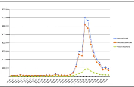
For the first year of simulation (2008) regression models were applied (see 14, 15). After 2008 scenario techniques are introduced in order to estimate the spatial effects of the crisis as well as the expected overall development of the German districts (see 16, 17). Three scenarios have been considered: most optimistic development, expected development and pessimistic development of some influencing variables like the development of the number of short time workers, the changes in the wages, to mention a few. In the following the assumptions, hypotheses and results related to the most optimistic scenario are presented, since a comparison with empirical data of the years 2008 and 2009 shows that the economic crisis for Germany was less dramatic as expected (see Figure 5) and had merely lead to a stagnation in the economic output.
Assumptions and hypotheses (used optimistic scenario):
In March 2009 more than 700.000 short-time workers are registered in Germany. It is assumed that a part of the short-time jobs are transferred into unemployment, depending on the job-qualification level and the branches of the industry.
The economic crash has an impact on the development of the regional wage level. It is assumed that in 2009 the regional wage levels are stagnating and start in 2010 to increase again, with the rate before the crisis.
Furthermore, a slow increase of productivity is assumed. This may - in the long run - lead to a reduction of the number of jobs.
It is assumed that in 2010 the situation on the labour market and the number of unemployed on average is rising to 4.1 million (Ifo, 2009).
Figure 1. View of short-time-work activities (employees), source: IAB
-100.000 200.000 300.000 400.000 500.000 600.000 700.000 800.000
Jan 07 Feb
07 Mrz
07 Apr
07 Mai
07 Jun
07 Jul 0
7 Aug 0
7 Sep 0
7 Okt
07 Nov
07 Dez
07 Jan
08 Feb
08 Mrz
08 Apr
08 Mai
08 Jun
08 Jul 0
8 Aug 0
8 Sep 0
8 Okt
08 Nov
08 Dez
08 Jan
09 Feb
09 Mrz
09 Apr
09 Mai
09 Jun
09 Jul 0
9 Aug 0
9 Sep 0
9 Okt
09
Deutschland Westdeutschland Ostdeutschland
The wages per day WpTi(t) are estimated via a multiple regression (14). Beside the wages of the previous year, the change of the gross-domestic product ∆BIP(t−1), and the GINI-coefficient GINI(t−1)concerning the yearly regional income distribution and a dummy variable to distinguish between East or West German districts are of importance. The GINI-coefficient is used as a common measure of statistical dispersion, this means of regional inequality. The importance of spatial autocorrelation measures and measures of inequality for the understanding of regional development, especially of regional employment is discussed e.g. in Zierhahn (2012).
(14)
The number of days of employment per capita TpBFi(t) is also calculated for the year 2008 via a multiple regression (15). As explanatory variables the rate of unemploymentALOQi(t−1), the GINI-coefficient GINI(t−1), the wages per day WpTi(t) and the workplace density become significant.
(15)
For the forecasting period after 2008 different modelling approaches and heuristic assumptions (time series) have been applied (16, 17)
(16)
(17)
In Figure 2 the development of the average wages per day WpTi(t)in East and West Germany are shown. Empirical data exist until 2007 (vertical line), then forecasting starts. These curves are obtained via averaging over all West German and East German districts in order to show the overall development of the average wages per day of West and East Germany and Germany as a whole.
)) 1 ( ),
1 ( ),
1 ( ,
) 1 ( ( )
(t =hWpT t− GINI t− ∆BIP t− EF t−
WpTi AO i AO i i iAO
)) 1 ( ),
1 ( ), 1 ( ),
1 ( (
)
(t =q ALOQ t− GINI t− LpT t− workplacedensity t−
TpBi AO i i i
,...) ) 1 ( ( )
( AO i AO
i t f WpT t
WpT = −
,...) ) 1 ( ( )
( AO i AO
i t g TpB t
Figure 2. Development of the average wages per day of Germany (2004 to 2007 empirical data, 2008 to 2015 simulated data), source: STASA
95% 98% 100% 103% 105% 108% 110% 113% 115%
2004 2005 2006 2007 2008 2009 2010 2011 2012 2013 2014 2015
year
W
a
g
e
s
p
e
r
d
a
y
W
p
T
West Germany Germany
East Germany
95% 98% 100% 103% 105% 108% 110% 113% 115%
2004 2005 2006 2007 2008 2009 2010 2011 2012 2013 2014 2015
year
W
a
g
e
s
p
e
r
d
a
y
W
p
T
West Germany Germany
East Germany
In Figure 3 the development of the days of employment per year are depicted. The economic upswing between 2004 and 2007 has lead to an increase in the average number of working days per year of about 2% in East Germany and stopped the decrease in the number of working days in West Germany. The economic crisis in 2008 and 2009 forced a reduction in the working days by almost 1.5% in East and 1.0% in West Germany. Starting with 2011 the number of working days per year indicates a smart recovering approaching the values of 2007-2008 around the year 2014.
Figure 3. The development of the days of employment per year (2004 to 2007 empirical data, 2008 to 2015 simulated data), source: STASA
95% 96% 97% 98% 99% 100% 101% 102% 103%
2004 2005 2006 2007 2008 2009 2010 2011 2012 2013 2014 2015
year
D
e
v
e
lo
p
m
e
n
t
T
p
B
a
o
i
n
%
East Germany
West Germany Germany
95% 96% 97% 98% 99% 100% 101% 102% 103%
2004 2005 2006 2007 2008 2009 2010 2011 2012 2013 2014 2015
year
D
e
v
e
lo
p
m
e
n
t
T
p
B
a
o
i
n
%
East Germany
West Germany Germany
95% 96% 97% 98% 99% 100% 101% 102% 103%
2004 2005 2006 2007 2008 2009 2010 2011 2012 2013 2014 2015
year
D
e
v
e
lo
p
m
e
n
t
T
p
B
a
o
i
n
%
East Germany
West Germany Germany
Figure 4. Development of the volume of employment of Germany (2004 to 2007 empirical data, 2008 to 2015 simulated data), source: STASA
92% 94% 96% 98% 100% 102% 104% 106%
2004 2005 2006 2007 2008 2009 2010 2011 2012 2013 2014 2015
year D e v e lo p m e n t o f B V a o % West Germany Germany East Germany 92% 94% 96% 98% 100% 102% 104% 106%
2004 2005 2006 2007 2008 2009 2010 2011 2012 2013 2014 2015
year D e v e lo p m e n t o f B V a o % West Germany Germany East Germany
The reduction in the total volume of employment and the development of the wages determine the temporal evolution of the gross wage payment (Figure 5).
Figure 5. Development of the gross wage payment of Germany (2004 to 2008 empirical data, 2008 to 2015 simulated data), source: STASA
95% 100% 105% 110% 115% 120%
2004 2005 2006 2007 2008 2009 2010 2011 2012 2013 2014 2015
year D e v e lopm e n t of gr os s -w a g e -pa y m e nt a t th e pl a c e of w or k East Germany West Germany Germany 95% 100% 105% 110% 115% 120%
2004 2005 2006 2007 2008 2009 2010 2011 2012 2013 2014 2015
year D e v e lopm e n t of gr os s -w a g e -pa y m e nt a t th e pl a c e of w or k East Germany West Germany Germany 95% 100% 105% 110% 115% 120%
2004 2005 2006 2007 2008 2009 2010 2011 2012 2013 2014 2015
year D e v e lopm e n t of gr os s -w a g e -pa y m e nt a t th e pl a c e of w or k East Germany West Germany Germany
3. Forecasted spatial interdependencies: example Bavaria
In order to show the impact of the crises on spatial structure, the development of the expected trajectories on the district level without crises will be compared with the expected trajectories with crises using scenario technique. It is assumed, that on the basis of multiple regression results the regional attractiveness indicators (8) to migrate, as well as the variables wages per day (14, 16) and working hours per day (15, 17) can be appropriately estimated for all 413 districts. Moreover, the impacts of the crises are superimposed by redistribution effects not related to the crises, e.g. by events planned on the long-run. In addition assumptions concerning cross-boarder migration have to be implemented. Here we follow in part the assumptions used by the Statistische Bundesamt, Wiesbaden.
Based on experience it is reasonable to assume that positive/negative economic effects must exist over a longer time period in order to be considered in the decision process of employees to migrate. Therefore, the effects of the crises on population distribution as well as related economic impacts will be considered after a cumulating period of 5 years. Furthermore it is assumed that only a part of the population, roughly estimated about 10% (part of the population with appropriate characteristics) will consider the impacts of the crises in its decisions to migrate. For all others no changes in its migration behaviour are expected. The development of the different districts of Bavaria is based on the following classification scheme for the cluster identification:
• Population development: < -0.1%
• Population development: > +0.1%
• Population development: -0.1% and + 0.1%
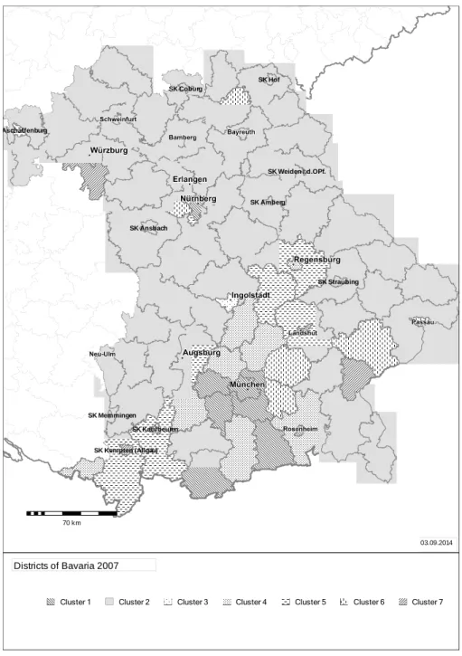
A comparison of the expected development of the different districts without crises and with crises yields therefore 9 possible clusters. However only 7 types of clusters can be identified (see Figure 6):
Cluster 1: Growth of population increased by the crises
Districts belonging to this cluster are the motors of Bavaria: Munich City, Augsburg City, Nuremberg City, and some others.
Cluster 2: Loss of population increased by the crises
Many smaller cities and rural districts belong to this cluster: Wunsiedel, Coburg, Cham, Bayreuth, Ansbach, to mention a few.
Cluster 3: Strong growth of population will be stopped by the crises
Only one district, namely the City of Ingolstadt belongs to this cluster. Especially Ingolstadt depends strongly on car industry (Audi) and related sectors. Since in Germany especially the car sector was mostly affected by the crises, it is reliable that this region will loose high qualified employees due to labour force migration.
Cluster 4: Growth of population will be diminished by the crises
Districts of this cluster are Fürth City, Freising, Bad Tölz, Dachau, Rosenheim, Landsberg, Lindau and a few more. The positive population increase of these districts will be diminished due to the impacts of the crises, but will stay positive.
The crises enforce out migration of population in the long-run, leading to a negative population balance. The districts are Erlangen City, Regensburg, Schweinfurt City, Kelheim, Aschaffenburg City, Landshut, Ostallgäu, to mention a few.
Cluster 6: Population development not affected by the crises
To this cluster belong the more rural districts Erding, Ebersberg, Passau, Fürth, Rottal-Inn, Kulmbach and Kaufbeuren.
Cluster 7: Population gain due to the crises can not compensate the losses due to out migration
Migration events influenced by the crises have a positive impact on the population balance of these districts and reduce the expected out migration. This cluster is build by the districts Wuerzburg, Altoetting, Kempten, Hof and Bayreuth City.
4. Conclusions
The complexity of forecasts at the regional level requires not only the involvement of many endogenous and interrelated variables and an appropriate modelling of the corresponding driving forces but also the possibility to introduce exogenous shocks. Of course, labour force migration and commuting are influenced by the development of the economy. However, the inertia of migration processes lead to a delayed reaction of the labour force on the crises.
In order to demonstrate the impact of the crises on the spatial interdependencies between districts of Germany the development of the expected trajectories on district level with and without crises are compared. Multiple regressions are used to model the driving forces of the process for all 413 German districts.
Figure 6. Expected impacts of the current economic crises on population development of Bavaria (district level).
Baden-Württemberg Hessen
Thüringen
Bayern
SK Kempten (Allgäu) SK Memmingen
SK Kaufbeuren SK Ansbach
SK Coburg
SK Aschaffenburg
SK Hof
SK Weiden i.d.OPf.
SK Amberg
SK Straubing
70 km
03.09.2014
Cluster 1 Cluster 2 Cluster 3 Cluster 4 Cluster 5 Cluster 6 Cluster 7
Districts of Bavaria 2007
Acknowledgements. Our special thanks go to K. Lichtblau and our former colleague M. Koller for many deep going discussions on regional development and job qualification.
References
Baas, T. (2014) Migration, in Braun, N. and Saam, J.N. (eds.) Handbuch Modellbildung und Simulation in den Sozialwissenschaften, Springer, Heidelberg.
Baas, T. and Brücker, H. (2012) The macroeconomic consequences of migration diversion: evidence for Germany and the UK, Structural Change and Economic Dynamics, 23(2), 180-194.
Bade, F.J. and Niebuhr, A. (1999) Zur Stabilität des räumlichen Strukturwandels, Jahrbuch
Blien, U. and Hirschenauer, F. (1999) Regionale disparitäten auf ostdeutschen
Arbeitsmärkten, in Wiedemann, E. et al. (eds.) Die arbeitsmarkt- und
beschäftigungspolitische Herausforderung in Ostdeutschland, Beiträge zur Arbeitsmarkt- und Berufsforschung, Bundesanstalt für Arbeit, Bd. 223.
Blien, U. (1998) Arbeitslosigkeit und Entlohnung auf regionalen Arbeitsmärkten,
Habilitationsschrift, Nürnberg.
Binder, J., Haag, G. and Koller, M. (2002) Modelling and simulation of migration, regional
employment development and regional gross wage payment in Germany: the bottom-up approach, paper presented in Regional Economies in Transition, Uddevalla
Symposium 2001, Vänersborg.
Birg, H. (1979) Zur Interdependenz der Bevölkerungs- und Arbeitsplatzentwicklung,
DIW-Sonderheft 131, Dunker und Humbolt, Berlin.
Björn, A., Mitze, T. and Untiedt, G. (2010) Internal migration, regional labour market dynamics and implications for German East-West disparities: results from a panel VAR, Jahrbuch der Regionalwissenschaften, 30(2), 159-189.
Bundesagentur für Arbeit (2008) Der Arbeits- und Ausbildungsmarkt in Deutschland, Monatsbericht Dezember und das Jahr 2008. Nürnberg.
Domencich, T.A. and McFadden, D. (1975) Urban travel demand: a behavioural analysis, North-Holland, Amsterdam.
Fazio, R.H. and Zanna, M.P. (1981) Direct experience and attitude-behaviour consistency, in Berkovitz, L. (ed.) Advances in Experimental Social Psychology, 51, 161-202.
Fechner, G.T. (1877) In Sachen der Psychophysik, Breitkopf und Härtel, Leipzig. Franz, W. (1997) Arbeitsmarktökonomik, Springer, Berlin, Heidelberg.
Fischer, M., Haag, G., Sonis, M. and Weidlich, W. (1988) Account of different views in
dynamic choice processes, WSG Discussion Paper 1/88, Wirtschaftsuniversitaet Wien.
Haag, G. and Weidlich, W. (1984) A stochastic theory of interregional migration,
Geographical Analysis, 16(4), 331-357.
Haag, G. (1989) Dynamic decision theory: application to urban and regional topics, Dordrecht, Kluwer Academic Publishers.
Koller, M., Schwengler, B. and Zarth, M. (2001) Efficency analysis for regional policies in
Germany (Zielerreichungsanalyse), IAB-Beiträge zur Arbeitsmarkt- und Berufsforschung, Bd. 243.
Koller, M. and Schwengler, B. (1999) Revisal and selection of German regions for structural
subsidies (Arbeitsmarkt- und Einkommensindikatoren), Expert Report presented to the
National Commission in March 1999, in Mitteilungen aus der Arbeitsmarkt- und Berufsforschung: Vorranggebiete der regionalen Arbeitsmarkt- und Strukturpolitik, 564-602, (1999) and in: Beiträge zur Arbeitsmarkt- und Berufsforschung: Struktur und Entwicklung von Arbeitsmarkt und Einkommen in den Regionen, No. 323 (2000). Nijkamp P. (ed.) (1985) Technological change, employment and spatial dynamics, Lecture
Notes in Economics and Mathematical Systems, 270, Springer.
Tassinopoulos, A. (2000) Die prognose der regionalen Beschäftigungsentwicklung, Beiträge
zur Arbeitsmarkt- und Berufsforschung, Bundesanstalt für Arbeit, Bd. 239.
Weber, A. (1909) Über den Standort der Industrien, Tübingen.
Weidlich, W. and Haag, G. (ed.) (1988) Interregional migration, Springer, Berlin.