NONPARAMETRIC BAYES METHODS FOR HIGH DIMENSIONAL DATA AND GROUP SEQUENTIAL DESIGN FOR LONGITUDINAL
TRIALS
Jing Zhou
A dissertation submitted to the faculty of the University of North Carolina at Chapel Hill in partial fulfillment of the requirements for the degree of Doctor of Philosophy in
the Department of Biostatistics.
Chapel Hill 2014
Approved by:
Amy H. Herring
David B. Dunson
Gary Koch
c 2014 Jing Zhou
ABSTRACT
JING ZHOU: Nonparametric Bayes Methods for High Dimensional Data AND Group Sequential Design for Longitudinal Trials
(Under the direction of Amy H. Herring)
High-dimensional unordered categorical data appear in a number of areas ranging from epidemiology, behavioral and social sciences, etc. Such data can be placed into a large contingency table with cell counts defined as the number of subjects with a given combination of variables values. The contingency table is often sparse in prac-tice in the sense that only a few cells have more than a few counts, with most cells being empty. Traditional approaches for contingency table analysis fail to scale up to moderate dimensions, and alternative approaches based on tensor decomposition are promising. This motivates us to develop sparse tensor decompositions for multivariate categorical variables where the number of variables can be potentially larger than the sample size. The methods are shown to have excellent performance in simulations, and results in various data sets are presented.
are shown to have higher power and lower false discovery rates in simulation studies relative to existing methods, and we consider an application to an epidemiologic study of birth defects.
ACKNOWLEDGMENTS
First and foremost I want to thank Professor Amy Herring for all of her valuable guidance and support through my years at UNC-Chapel Hill. I do not think I could have had a better example of how to perform quality research and carry oneself as a professional.
I am grateful to Prof. David Dunson for his suggestions and feedback on multiple projects over the course of my studies, and to Anirban Bhattacharya for being a great research colleague.
I also want to thank Prof. Gary Koch, Dr. Keaven Anderson, and Prof. Andrew Olshan for serving on my Ph.D. committee and for their helpful input and suggestions. I appreciate Dr. Keaven Anderson for providing a very interesting research topic to expand my research horizons.
My research would not have been possible without the financial support of the National Birth Defects Prevention Study grant. I am also grateful to the research team in providing great scientific support.
TABLE OF CONTENTS
LIST OF TABLES. . . ix
LIST OF FIGURES . . . x
1 Literature Review . . . 1
1.1 Bayesian Methodologies Introduction(Paper 1 and 2) . . . 1
1.1.1 Dirichlet Distribution and Process . . . 5
1.1.2 Tensor Decomposition . . . 8
1.1.3 Bayes Nonparametrics . . . 9
1.1.4 Joint and Conditional Probabilistic Modeling . . . 10
1.2 Sample Size Re-estimation Introduction(Paper 3) . . . 13
2 Sparse Tensor Factorizations for Big Contingency Tables . . . 17
2.1 Introduction . . . 17
2.2 Sparse Factor Models for Tables . . . 20
2.2.1 Model and prior . . . 20
2.2.2 Induced prior in log-linear parameterization . . . 24
2.3 Posterior Computation . . . 25
2.4 Simulation Studies . . . 27
2.4.1 Estimating sparse interactions . . . 27
2.4.2 Comparison with standard PARAFAC . . . 30
2.5 Application . . . 30
2.5.1 Splice-junction Gene Sequences . . . 30
2.5.3 National Birth Defects Prevention Study . . . 32
2.6 Discussion . . . 33
3 Nonparametric Bayes Modeling for Case Control Studies . . . 50
3.1 Introduction . . . 50
3.2 Conditional Sparse Parallel Factor Analysis Model . . . 53
3.2.1 Model and prior . . . 53
3.2.2 Inference . . . 58
3.3 Posterior Computation . . . 58
3.4 Simulation Studies . . . 60
3.4.1 Simulation from log-linear models . . . 60
3.4.2 Simulation from latent class models . . . 62
3.5 Application to the National Birth Defects Prevention Study . . . 64
3.6 Discussion . . . 68
4 Sample Size Re-estimation in Longitudinal Group Sequential Design 82 4.1 Outline . . . 82
4.2 Sample Size Determination for Longitudinal Analysis . . . 82
4.2.1 Model Notation . . . 82
4.2.2 Fixed Design . . . 84
4.2.3 Group Sequential Design . . . 85
4.3 Information-Based Sample Size Re-Estimation . . . 87
4.3.1 Sample Size Re-estimation . . . 87
4.3.2 Adaptation . . . 88
4.3.3 Interim Analysis Procedure . . . 91
4.4 Simulation Study . . . 92
4.6 Discussion . . . 97
Appendix I: List of Significant Associations - Birth Defects Study . . 114
Appendix II: Computation Code for Chapter 2 . . . 128
Appendix III: Computation Code for Chapter 3 . . . 136
Appendix IV: Computation Code for Chapter 4 . . . 145
LIST OF TABLES
2.1 Summary statistics of induced priors on coefficients in log-linear model
parameterization. . . 47
2.2 Power for Non-null Variables Based on 100 Simulations . . . 48
2.3 Type I Error for Null Variables Based on 100 Simulations . . . 49
3.1 True Coefficients . . . 77
3.2 True Coefficients (continued) . . . 78
3.3 True Coefficients for Another Four Dependent Variables . . . 79
3.4 Power Using 95% Credible Intervals . . . 80
3.5 Type I Error Using 95% Credible Intervals . . . 81
4.1 Simulation Error . . . 109
4.2 Power Based on Varying Correlation Coefficients . . . 110
4.3 Type I Error Based on Varying Correlation Coefficients . . . 111
4.4 Longitudinal Data with Four visits . . . 112
LIST OF FIGURES
2.1 Histograms of induced priors for one main effect β1, one two-way
inter-action β12, and the three-way interactionβ123 - Top Row: γ = 1; Middle
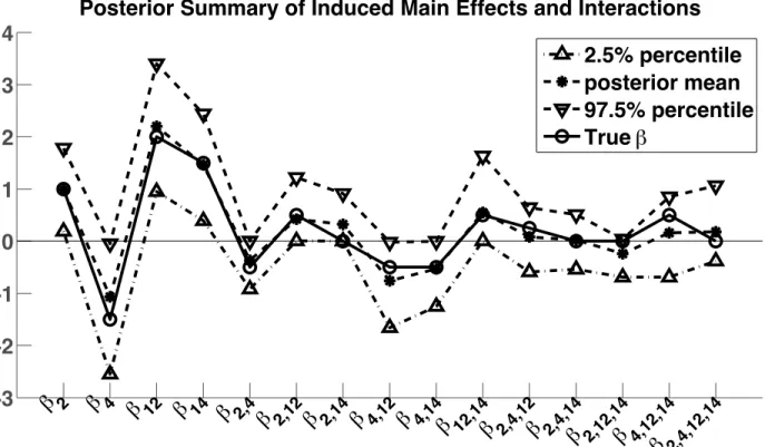
Row: γ = 5; Bottom Row: γ = 20. . . 35 2.2 Posterior means and 95% credible intervals for all main effects and
in-teractions in S∗ compared with the true coefficients. . . 36 2.3 Left: Posterior summaries of the Cramer’s V values for all dependent
pairs vs. the true Cramer’s V values; Right: Estimated density of Cramer’s V combining all null pairs under sp-PARAFAC vs. empiri-cal estimation. . . 37
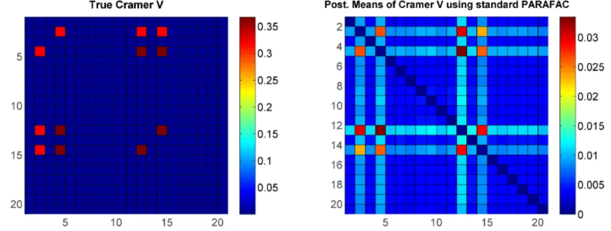
2.4 Simulation setting (i) – Left: True Cramer’s V matrix; Right: Posterior means of Cramer’s V using standard PARAFAC. Top 20×20 sub-matrix shown. . . 38
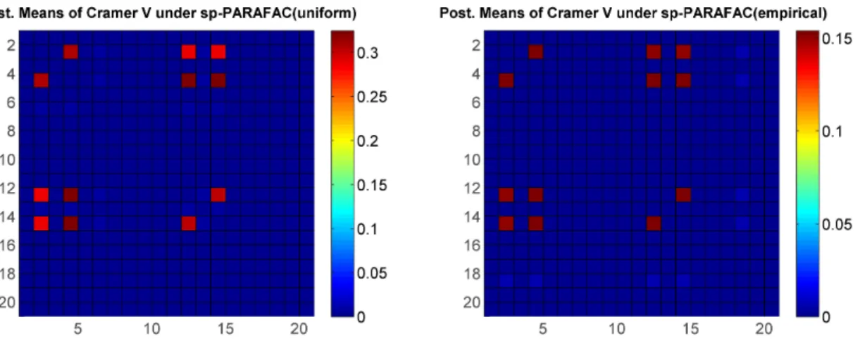
2.5 Posterior means of Cramer’s V under simulation setting (i) using pro-posed method – Left: with λ(0j) being discrete uniform; Right: with λ(0j) being empirical estimates of the marginal category probabilities. Top 20×20 sub-matrix shown. . . 39
2.6 Posterior means of Cramer’s V under simulation setting (ii) – Left: using standard PARAFAC; Middle: under proposed method using empirical marginal with Diri(1,...,1) prior for λ0; Right: using proposed method
with discrete uniform λ0. Top 20×20 sub-matrix shown. . . 40
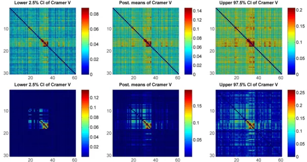
2.7 Posterior quantiles of Cramer’s V with 120 sequences of splice data – Upper panel: under standard PARAFAC; Bottom panel:under proposed method. . . 41
2.8 Posterior quantiles of Cramer’s V with 3,175 sequences of splice data – Upper panel: under standard PARAFAC; Bottom panel:under proposed method. . . 42
2.9 Posterior quantiles of Cramer’s V with 100 subjects of PUMS – Upper panel: under standard PARAFAC; Bottom panel: under proposed method. 43
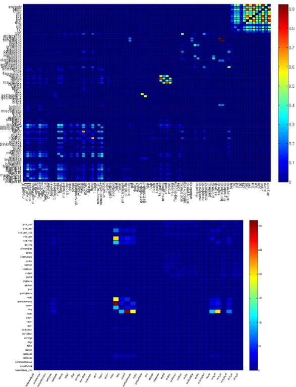
2.11 Upper panel:Posterior mean of Cramer’s V for 80 potential factors; Bot-tom panel: Posterior mean of significant odds ratios within 37 heart related birth defects. . . 45
2.12 Upper panel: Posterior mean of odds ratios between 37 heart related birth defects and 80 potential factors; Bottom panel: Posterior mean of odds ratios between 2 cleft defects and 80 potential factors. . . 46
3.1 ROC curves under loglinear true models – Left: p=20; Right: p=100. . 70
3.2 ROC curves under loglinear true models with more correlated covariates – Left: p=20; Right: p=100. . . 71
3.3 ROC curves under latent class true models – Left: p=20; Right: p=100. 72
3.4 ROC curves under latent class true models with more correlated covari-ates – Left: p=20; Right: p=100. . . 73
3.5 Part 1 – significant odds ratios between 19 birth defects and 64 potential factors. Top: using proposed method; Bottom: using 1-to-1 logistic regression. . . 74
3.6 Part 2 – significant odds ratios between 19 birth defects and 64 potential factors. Top: using proposed method; Bottom: using 1-to-1 logistic regression. . . 75
3.7 Part 3 – significant odds ratios between 19 birth defects and 64 potential factors. Top: using proposed method; Bottom: using 1-to-1 logistic regression. . . 76
4.1 Adaptation Example . . . 100
4.2 Power Curves Using Our Re-estimation Method (Left) v.s. Fixed Design (Right) . . . 101
4.3 Left: Power Curves Using Group-sequential Design without Re-estimation; Right: Expected Sample Size Using Group Sequential Design with Sam-ple Size Re-estimation v.s. Fixed Design . . . 102
4.5 Left: Type-I Error Using Group-sequential Design without Re-estimation; Right: Expected Sample Size Using Group Sequential Design with Sam-ple Size Re-estimation v.s. Fixed Design . . . 104
4.6 Simulations Results Based on the Last Time Point Only Using the Method by Mehta and Tsiatis (2001) . . . 105
4.7 Simulation Results Based on the Last Time Point Only Using the Method by Mehta and Tsiatis (2001) (continued) . . . 106
4.8 Simulation Results Based on the Last Time Point Only Using the Method by Mehta and Tsiatis (2001) (continued) . . . 107
CHAPTER 1 Literature Review
1.1 Bayesian Methodologies Introduction(Paper 1 and 2)
The most important aspects of epidemiologic research are uncovering dependencies among multiple closely-related exposures and health outcomes, discovering risk factors, and developing accurate predictive models. This is particularly true given that it is crucial in many settings to account for interactions. Multivariate unordered categorical data are routinely encountered in such areas. For example, the categorical variables may correspond to a sequence of A, C, G, T nucleotides in candidate genes or responses to questionnaire data on race, religion and demographic information for an individual (Bhattacharya and Dunson 2012).
collinearity among variables and sparsity of the cells. Hence, it is not possible simul-taneously to obtain an estimate (e.g., odds ratio) for each cell of the table without borrowing information strongly. To address this, one could typically apply dimen-sionality reduction techniques such as (1) preselect variables that seem likely to be important and ignore interactions to reduce dimensionality; (2) group exposures into class-specific summaries; or (3) include variables one at a time as predictors in a low-dimensional logistic regression model, with interactions only added for predictors with main effects, and significance thresholds on p-values adjusted for false discovery rate control. However, such approaches can lead to (1) overlooking important risk factors; (2) discarding valuable information on variability in the effect within a class; or (3) producing misleading results by not adjusting for correlated exposures. Furthermore, it lacks a probabilistic characterization of uncertainty, which is important in making inferences and representing uncertainty in predictions.
(2012).
For unordered categorical variables, factor models, however, run into computation problems due to their complex model and estimation nature. But the data could be alternatively presented in the form of a high-dimensional contingency table for which there is a vast literature. Fienberg and Rinaldo (2007) provide an overview of the de-velopment of log-linear models, maximum likelihood estimation and asymptotic tests for goodness of fit. While log-linear models provide a framework to model interac-tions among related categorical variables, the number of model parameters becomes large even in the case of a two-way interaction model for moderate to large number of variables. Asymptotic tests based on log-linear models face multiple difficulties in the case of sparse contingency tables –refer to the discussion in section 3 of Fienberg and Rinaldo (2007). Although such problems can be alleviated using a Bayesian approach, posterior model search using traditional Markov chain Monte Carlo (MCMC) methods tends to slow down quickly as the dimension increases. Moreover, even with highly effi-cient search algorithms (Jones et al. 2005; Carvalho and Scott 2009; Dobra and Massam 2010), it is only feasible to visit a small subset of the model space even for moderate pand accurate model selection is a difficult task. This motivates the development of a new class of models for high-dimensional unordered categorical data in the form of a contingency table.
related to non-negative tensor decompositions (Shashua and Hazan 2005; Kim and Choi 2007).
Likewise, Yang and Dunson (2013) proposed a different nonparametric Bayes model on the conditional distribution of the category probabilities. By choosing a carefully-structured Tucker factorization, another popular tensor decomposition method, they defined a model that can characterize any conditional probability, while facilitating variable selection and modeling of high-order interactions. They suggested a two-stage algorithm which first identifies a model with a set of important predictors in the first stage and then learns the posterior distribution for this model via the Gibbs sampler for other unknown parameters.
1.1.1 Dirichlet Distribution and Process Dirichlet Distribution
The basic building tool for Bayesian non-parametric methods is called the Dirichlet Process (DP). To discuss the Dirichlet process, we first need to discuss the Dirichlet distribution. The Dirichlet distribution is the multivariate generalization of the beta distribution. Let z1, . . . , zk be independent random variables with zj ∼Gamma(aj,1), j = 1, . . . , k. Define
u= k X j=1 zj, and
yj = zj
u = zj
Pk
j=1zj
.
Since Pk
j=1yj = 1, we say (y1, . . . , yk) have ak−1 dimensional Dirichlet distribution
Dk−1(a1, . . . , ak) with density
f(y1, . . . , yk) =
Γ(Pk
j=1aj)
Qk
j=1Γ(aj)
k
Y
j=1
yaj−1
j
.
The Dirichlet distribution is a distribution over possible vectors for a multinomial dis-tribution. It is in fact a ’distribution over distributions’ and hence can be used as a conjugate prior for the multinomial family. That is, if
(x1, . . . , xk)∼Multinomial(p1, . . . , pk), where k
X
j=1
pj = 1,
then the conjugate prior for (p1, . . . , pk) is Dk−1(a1, . . . , ak). The posterior, as a result, has the form,
wherex= (x1, . . . , xk).
Dirichlet Process
A Dirichlet process, DP(αG0), expressed as G is with base distribution G0 and
scale parameter α. G is a random probability measure that has the same support as G0. It is also a distribution over distributions. Ferguson (1973) introduced the
Dirichlet process as a class of prior distributions for which the support is large, and the posterior distribution is analytically manageable. The idea of using a Dirichlet process as the prior for the mixing proportions of a simple distribution (e.g., Gaussian) was first introduced by Antoniak (1974).
Consider a model with a parametric likelihood: yi ∼N(θi, τi−1). Instead of assuming θi ∼G0, we could specifyθi ∼G, andG∼DP(αG0), whereG0is the base distribution
such as a normal distribution andαis a precision parameter determining how closelyG followsG0. The Dirichlet process (DP) model is simplified in practice by the Polya urn
representation (Blackwell and MacQueen 1973). It relies on marginalizing out G to obtain
(θi|θ1, . . . , θi−1)∼
α
α+i−1)G0+ i−1
X
j=1
1 α+ 1
δθj. (1.1)
It can be seen that the θi’s are distributed as the base measure along with the added property that P(θi = θj) > 0 for i 6= j. The Dirichlet process prior results in what MacEachern (1994) calls a cluster structure among the θi’s. This cluster structure partitions the n θi’s into k sets or clusters, 0 < k ≤ n. All of the observations in a cluster share an identical value of θ and subjects in different clusters have different values of θ.
in-patrons of the restaurant. Let
1. 1st customer sits at table with dish ζ
1;
2. 2nd customer sits at first table with probabilityα/(1 +α) or new table with dish ζ2 with probability 1/(1 +α);
3. process encourages later customers to sit at well occupied tables.
We can see from (1.1) that a customer is more likely to sit at a table if there are already many people sitting there. However, with probability proportional to α, the customer will sit at a new table.
Another popular way of presenting DP, introduced by Sethuraman (1994), is called the stick-breaking process:
θi ∼G=
∞
X
h=1
νhδθh,
where
νh =Vh
Y
l<h
(1−Vl), Vh ∼Beta(1, α), θh ∼G0,
for h = 1, . . . ,∞, with δθ denoting the degenerate distribution with all its mass at θ. One can illustrate this by starting from a unit probability stick,
1. Break off a random piece (V1) and allocate this to a random value (θ1);
2. From the remaining 1−V1, break off a proportion V2 and allocate toθ2;
3. Repeat infinitely many times.
Compared with the Polya urn scheme, the stick-breaking process is more attractive in the sense that it provides the ability to conduct inference onG by avoiding marginal-ization ofG.
from the posterior distribution of the parameters of the component distributions and/or of the associations of mixture components with observations. Methods based on Gibbs sampling can easily be implemented for models based on conjugate prior distributions.
1.1.2 Tensor Decomposition
LetTd1...dpdenote the set of all tensors of dimensiond1×. . .×dp, andΠd1...dp ⊂Td1...dp
denote the set of all probability tensors, so thatπ ∈Πd1...dp implies
π =
πc1...cp ≥0, cj = 1, . . . , dj, j = 1, . . . , p:
d1 X
c1=1
· · · dp X
cp=1
πc1...cp = 1
.
One way of tensor generalization of the matrix singular value decomposition is called PARAFAC decomposition (Harshman 1970; Harshman and Lundy 1994; Zhang and Golub 2001). Kolda (2001) used the notation
D= k
X
h=1
λhUh, Uh =u
(1)
h ⊗u
(2)
h ⊗ · · · ⊗u
(p)
h ,
where λ1 ≥ · · · ≥ λk > 0, Uh is a decomposed tensor with u
(j)
h ∈ <dj, and ⊗ denotes the outer product, so that
Dc1...cp =
k
X
h=1
λhu
(1)
hc1. . . u
(p)
hcp.
One definition of the rank of a tensor is the minimal k such that D can be expressed as a sum ofk decomposed (or rank one) tensors.
tensor D∈Td1...dp as
Dc1...cp =
d1 X
h1=1
· · · dp X
hp=1
gh1...hpu
(1)
h1c1. . . u
(p)
hpcp,
where G={gh1...hp} ∈ Td1...dp is called a core tensor and its entries control interaction
between the different components. Wang and Ahuja (2005); Kim and Choi (2007) and Yang and Dunson (2013) empirically noted that the HOSVD achieves better data compression and requires fewer components compared to the PARAFAC model as it uses all combinations of the mode vectorsu(hj)
j’s,h = 1, . . . , k.
With an interest in decomposing a probability matrix/tensor, the non-negative ma-trix factorization (NMF) (Gregory and Pullman 1983; Cohen and Rothblum 1993) seeks the best approximation of a non-negative matrix A ∈ <m×n
+ as a product of
non-negative matrices W ∈ <m+×k and V ∈ <k+×n for some k ≤ min{m, n}, and finds the so-called non-negative rank as the minimal k such that a non-negative matrix can be written as a sum of rank one non-negative matrices. The non-negative versions of the PARAFAC and HOSVD decompositions for tensors are discussed in Kim and Choi (2007) and Shashua and Hazan (2005).
1.1.3 Bayes Nonparametrics
Before turning to the non-parametric model, first consider the fully parametric situation. Supposeyi is anni×1 random vector indexed by thep×1 parameter vector θi, for eachi= 1, . . . , n. Suppose the θi have a prior distribution with hyperparameter θ0. That is, θi
i.i.d.
∼ G(·|θ0). If G(·|θ0) is a specified function, then this corresponds to
the fully parametric situation. The fully parametric situation can be described by two stages:
• Stage 2: (θi|θ0) = G(·|θ0),
where G(·|θ0) is a specified prior distribution, such as a normal, gamma, exponential,
beta, etc..
In many parametric likelihood models, we often wish to relax the assumption of a parametric prior on the parameters. A common method is to set the prior distribution to be random such as a Dirichlet process prior, which leads to mixtures of Dirichlet processes (MDP). MDP removes the parametric assumption onG(·|θ0), that isG(·|θ0)
is not known and thus no functional form is specified for G. Thus the MDP model has 3 stages
• Stage 1: (yi|θi)∼ (parametric likelihood),
• Stage 2: θi i.i.d.
∼ G (G unknown), • Stage 3: G|α0, G0 ∼DP(α0G0).
Thus the MDP model has 3 stages with the last stage being the DP specification. The specification given above is semi-parametric in the sense that a parametric likelihood specification is given in stage 1, and a non-parametric specification is given in stages 2 and 3. Some examples of Bayes semi-parametric methods can be found in MacLehose et al. (2007); Dunson et al. (2008). If we further relax the stage 1 to model the data using a probabilistic characterization of uncertainty while accounting for interaction, such as a tensor factorization, it becomes a Bayes nonparametric model because both the distribution of the data,yi, and the distribution of the parameterθ are nonparametric.
1.1.4 Joint and Conditional Probabilistic Modeling
incor-probabilistic version of PARAFAC tensor decomposition by representingπ as
πc1...cp = Pr(xi1 =c1, . . . , xip =cp) =
k
X
h=1
νhλ
(1)
hc1. . . λ
(p)
hcp, (1.2)
where ν = (ν1, . . . , νk)0 is a vector of mixture probabilities, zi ∈ {1, . . . , k} is a latent class index, Pr(xij =cj|zi =h) =λ
(j)
hcj is the probability of xij =cj given allocation of
individualito classh. xi = (xi1, . . . , xip)0 are assumed to be conditionally independent given zi. Marginalizing over the distribution of zi induces dependence among the p variables. Note that it is different from a usual PARAFAC decomposition because of the non-negativity constraints on ν and the λ(hj)’s. In this paper, it is proved that any multivariate categorical data distribution can be characterized as a finite mixture of product-multinomial distributions as in (1.2).
However, it is not straightforward to obtain a well-justified approach for estimation of k. Regular methods like maximum likelihood estimation would fail to converge due to the sparsity of the data even for a modest k, or otherwise would provide biased results if small k is chosen. These issues provide motivation for utilizing a Dirichlet process, which avoids selection of a single finite k, allowing the number of components that are occupied by individuals in the sample to grow with sample size. One can specify priors
λ(hj) ∼ Dirichelet(aj1, . . . , ajdj),
using stick-breaking representation for ν, (1.2) and (1.3) can be expressed in the fol-lowing hierarchical form:
xij|zi =h ∼ Multinomial (1, . . . , dj);λ
(j)
h1, . . . , λ (j)
hdj
, zi ∼
∞ X h=1 Vh Y l<h
(1−Vl)δh, Vh ∼ Beta(1, α),
λh(j)≡(λh(j1), . . . , λ(hdj)
j) ∼ Diri(aj1, . . . , ajdj). (1.4)
The Gibbs sampling algorithm can be performed in a straightforward fashion. Bhat-tacharya and Dunson (2012) instead applied a different decomposition method to model the joint probability for multivariate categorical data. In comparison, rather than in-vestigating the dependence structure among variables, Yang and Dunson (2013) estab-lished a conditional probabilistic Tucker factorization with the goals of classifying the response of interest as well as identifying a sparse subset of important predictors. That is,
Pr(yi =c|xi1 =c1, . . . , xip =cp) = k1 X
h1=1
· · · kp X
hp=1
λh1···hp(c)
p
Y
j=1
πh(j)
j(cj), (1.5)
with constraints Pd0
c=1λh1...hp(c) = 1 and Pkj
h=1π (j)
h (cj) = 1. The value of kj ∈ {1, . . . , dj} controls the number of parameters characterizing the impact of the jth predictor on the conditional probability, with kj = 1 implying that the jth predictor is excluded from the model. We can simplify the representation by introducing p latent class indicators zi1, . . . , zip for xi1, . . . , xip. The model can be rewritten as
yi|zi1, . . . , zip ∼ Multinomial({1, . . . , d0};λzi1,...,zip), (1.6)
zij|xij =cj ∼ Multinomial({1, . . . , kj};π
(j)
1 (cj), . . . , π
(j)
where λzi1,...,zip ={λzi1,...,zip(1), . . . , λzi1,...,zip(d0)}. Integrating out the latent class
indi-cators, the conditional probability of yi given (xi1, . . . , xip) matches the form in (1.5).
The Dirichlet distribution priors are chosen for λh1...hp and π
(j)(c
j) to maintain conju-gacy, while some well-specified discrete distribution are specified forkjfavoring sparsity. Refer to Yang and Dunson (2013) for deriving the corresponding posteriors. Although it seems to have better prediction performance than existing methods and it has the capability of interpreting the relationship between predictors and the outcome, it is worth noting that the approximation of marginal likelihood of k = {k1, . . . , kp} was not justified in the paper and there are some computational issues when the number of variables with (kj >1) is bigger than seven.
In summary, both joint and conditional modeling have advantages of (i) allowing the distribution of multiple categorical variables to be unknown; (ii) a full proba-bilistic characterization of uncertainty accounting for any possible interaction among predictors; (iii) favoring a sparse structure that allows efficient computation without the problem of overfitting. Note that the joint model aims to infer the dependence structure among variables, while the conditional model focuses on the classification.
1.2 Sample Size Re-estimation Introduction(Paper 3)
(1) correlation among longitudinal visits; (2) standard deviation within longitudinal measurements for each subject and (3) retention rates in both treatment groups. For planning purposes, best guesses are made for the value of the nuisance parameters.
However, there is a great concern that these assumptions of nuisance parameters based on previous studies are often unreliable because of differences in the study pop-ulation, changes in medical practice, or the measurement techniques. Since incorrect assumptions can lead to substantial underpowering or overpowering to detect the clini-cally important difference, it may be prudent to check the validity of those assumptions using interim data from the study. There is a rich literature Coffey and Kairalla (2008); Chuang-Stein et al. (2006) discussing the sample size re-estimation methods to rescue the power. Wittes and Brittain (1990) introduced the concept of an internal pilot de-sign, which re-estimates the sample size in the mid-course of the study with no interim testing involved. Internal pilot designs have also been extended to different settings, besides normally distributed outcomes, such as repeated measures. Shih and Gould (1995) described a method to re-estimate sample size in the repeated measure frame-work. However it is only for a simplified setting, where the parameter of interest is the rate of change (slope) of a continuous measurement. Zucker and Denne (2002) extended Shih and Gould’s model to a general setting in which missing and dropout are allowed and a linear combination of treatment effect over time can be set as the meaningful difference to be detected.
CHAPTER 2
Sparse Tensor Factorizations for Big Contingency Tables
2.1 Introduction
Sparsely observed big tabular data sets are commonly collected in many applied domains. One example corresponds to recommender systems in which the dimensions of the table correspond to users, items and different contexts (Karatzoglou et al. (2010)), with a tiny proportion of the cells filled in for users providing rankings. The task is to fill in the rest of the huge table in order to make recommendations to users of which items they may prefer in each context. This extends the widely studied matrix completion problem (Cand`es and Recht (2009)) of which the Netflix challenge was one example. Another setting corresponds to contingency tables in which multivariate categorical data are collected for each individual, and the cells of the table contain counts of the number of individuals having a particular combination of values. In contingency table analyses, the focus is typically on inferring associations among the different variables, but challenges arise when there are many variables, so that the number of cells in the table is vastly bigger than the sample size.
Suppose that the tensor of interest is π ∈ Πd1×···×dp, with Πd1×···×dp a space of
Lee and Seung (1999); Friedlander and Hatz (2005); Lim and Comon (2009); Liu et al. (2012)). For contingency tables, the tensor corresponds to the joint probability mass function for multivariate categorical data, so that the elements are non-negative and add to one across all the cells (Dunson et al. (2008); Bhattacharya and Dunson (2012)). Let Y denote the data collected on tensor π. For recommender systems, Y consists of ratings for a small subset of the Qp
j=1dj cells in the tensor, while for contingency tables Y includes response vectors yi = (yi1, . . . , yip)T for subjects i = 1, . . . , n, with yij ∈ {1, . . . , dj} for j = 1, . . . , p. In both cases, data are extremely sparse, with no observations in the overwhelming majority of cells.
To combat this data sparsity, it is necessary to substantially reduce dimensionality in estimating π. The usual way to accomplish this is through a low rank assumption. Unlike for matrices, there is no unique definition of rank but the most common con-vention is to define the rank k of a tensor π as the smallest value ofk such that π can be expressed as
π = k
X
h=1
ψ(1)h ⊗ · · · ⊗ψh(p), (2.1)
which is sum ofkrank one tensors, each an outer product of vectors1 for each dimension
(Kolda and Bader 2009). Expression (1) is commonly referred to as parallel factor analysis (PARAFAC) (Harshman (1970); Bro (1997)). For k small, the number of parameters is massively reduced fromQp
j=1dj tok
Pp
j=1dj; as the low rank assumption often holds approximately, this leads to an effective approach in many applications, and a rich variety of algorithms are available for estimation.
However, the decrease in degrees of freedom from exponential inpto linear inpis not sufficient whenp is big. Largep smalln problems arise routinely, and a usual solution
1Forp= 2, ψ(1)⊗ψ(2) =ψ(1)ψ(2)T. In general, (ψ(1)⊗ · · · ⊗ψ(p))c1...cp=ψ(1)
c1 . . . ψ
outside of tensor settings is to incorporate sparsity. For example, in linear regression, many of the coefficients are set to zero (Tibshirani 1996; Scott and Berger 2010), while in estimation of large covariance matrices, sparse factor models are used that assume few factors and many zeros in the factor loadings matrices (West (2003); Carvalho et al. (2008)). In the matrix factorization literature, there has been consideration of low rank plus sparse decompositions (Chartrand (2012)), but this approach does not solve our problem of too many parameters. Including zeros in the component vectors {ψ(hj)} is not a viable solution, particularly as we do not want to enforce exact zeros in blocks of the tensor π but require an alternative notion of sparsity.
Our notion is as follows. For component h (h= 1, . . . , k), we partition the dimen-sions into two mutually exclusive subsets Sh∪Shc = {1, . . . , p}. The proposed sparse PARAFAC (sp-PARAFAC) factorization is then
π = k
X
h=1
ψh(1)⊗ · · · ⊗ψ(hp), ψh(j) =ψ0(j) for j ∈Sc
h. (2.2)
Hence, instead of having to introduce a separate vectorψh(j) for everyh andj, we allow there to be more degrees of freedom used to characterize the tensor structure in certain directions than in others. Consider the recommender systems application and suppose we have three dimensions, including users (j = 1), items (j = 2) and context (j = 3). If we let ψh(3) =ψ(3)0 for h= 1, . . . , k,
πc1c2c3 =ψ
(3) 0c3
k
X
h=1
ψhc(1)
1ψ
(2)
hc2, (2.3)
then the jth variable is independent of the other variables with Pr(yij = cj) = ψ
(j) 0cj.
By including j ∈ Shc for some but not all h ∈ {1, . . . , k} one can use fewer degrees of freedom in characterizing the interaction between the jth factor and the other factors. In practice, we will learn {Sh} using a Bayesian approach, as the appropriate lower dimensional structure is typically not known in advance.
We conjecture that many tensor data sets can be concisely represented via (2.2), with results substantially improved over usual PARAFAC factorizations due to the second layer of dimension reduction. For concreteness and brevity, we focus on con-tingency tables, but the methods are easily modified to other settings. Concon-tingency table analysis is routine in practice; refer to Agresti (2002); Fienberg and Rinaldo (2007). However, in stark contrast to the well developed literature on linear regression and covariance matrix estimation in big data settings, very few flexible methods are scalable beyond small tables. Throughout the rest of the paper, we assume that the ob-served datayi = (yi1, . . . , yip)T, i= 1, . . . , n, is multivariate unordered categorical, with yij ∈ {1, . . . , dj}. Our interest is in situations where the dimensionalitypis comparable or even larger than the number of samples n.
2.2 Sparse Factor Models for Tables
2.2.1 Model and prior
We focus on a Bayesian implementation of sp-PARAFAC in (2.2). LetSr−1 ={x∈
<r : xj ≥ 0,Pr
j=1xj = 1} denote the (r − 1)-dimensional probability simplex. In
the contingency table case, Dunson et al. (2008) proposed the following probabilistic PARAFAC factorization.
Pr(yi1 =c1, . . . , yip =cp) = πc1···cp =
k
X
h=1
νh p
Y
j=1
λ(hcj)
where ν = {νh} ∈ Sk−1 and λ
(j)
h = (λ
(j)
h1, . . . , λ (j)
hdj) ∈ S
dj−1 is a vector of probabilities
of yij = 1, . . . , dj in component h. Introducing a latent sub-population index zi ∈ {1, . . . , k}for subject i, the elements of yi are conditionally independent given zi with Pr(yij =cj |zi =h) = λ
(j)
hcj, and marginalizing out the latent indexzi leads to a mixture
of product multinomial distribution for yi. Placing Dirichlet priors on the component vectors leads to a simple and efficient Gibbs sampler for posterior computation. We will refer to this model (2.4) as standard PARAFAC.
This approach has excellent performance in small to moderatepproblems, but asp increases there is an inevitable breakdown point. The number of parameters increases linearly inp, as for other PARAFAC factorizations, so problems arise as p approaches the order of n or p n. For example, we are particularly motivated by epidemiology studies collecting many categorical predictors, such as occupation type, demographic variables, and single nucleotide polymorphisms. For continuous response vectors yi ∈ <p, there is a well developed literature on Gaussian sparse factor models that are
adept at accommodatingpndata (West (2003); Lucas et al. (2006); Carvalho et al. (2008); Bhattacharya and Dunson (2011)). These models include many zeros in the loadings matrices to induce additional dimension reduction on top of the low rank assumption. Pati et al. (2013) provided theoretical support through characterizing posterior concentration.
Our sp-PARAFAC factorization provides an analog of sparse factor models in the tensor setting. Modifying for the categorical data case, we let
πc1...cp =
k
X
h=1
νh
Y
j∈Sh
λ(hcj)
j Y
j∈Sc h
λ(0jc)
j, (2.5)
where|Sh| p(|S|denotes the cardinality of a set S) and theλ
(j)
advance; we consider two cases:
(i) λ(0j)=
1 dj, . . . ,
1 dj
T
and (ii) λ(0j) =
1 n n X i=1
1(yij = 1), . . . , 1 n
n
X
i=1
1(yij =dj)
T
,
corresponding to a discrete uniform and empirical estimates of the marginal category probabilities. By fixing the baseline dictionary vectors{λ(0j)}in advance, and allocating a large subset of the variables within each cluster h to the baseline component, we dramatically reduce the size of the model space. In particular, the probability tensor π in (2.5) can be parameterized as θπ = l(ν,{Sh}1≤h≤k,{λ
(j)
h }1≤h≤k,j∈Sh
˚), where ν ∈ Sk−1, S
h ⊂ {1, . . . , p}, λ
(j)
h ∈ Sdj
−1. Thus, the effective number of model parameters is
now reduced to (k−1) +Pk
h=1|Sh|+
Pk
h=1
P
j∈Sh(dj−1), which is substantially smaller
than the (k−1) + Pp
j=1k(dj −1) parameters in the original specification, provided |Sh| p for allh = 1, . . . k. The size of Sh is penalized via a sparsity favoring prior on |Sh|in (2.6) below. We will illustrate that this can lead to huge differences in practical performance.
Completing a Bayesian specification with priors for the unknown parameter vectors and expressing the model in hierarchical form, we have2
yij ∼Mult {1, . . . , dj};λ(zji)1, . . . , λ(zj)
idj
, λ(hj)∼(1−τh)δλ(j)
0
+τhDiri(aj1, . . . , ajdj),
Pr(zi =h) =νh =VhQl<h(1−Vl),
Vh ∼Beta(1, α), α∼Gamma(aα, bα), τh ∼Beta(1, γ). (2.6)
It is evident that the hierarchical prior in (2.6) is supported on the space of probabil-ity tensors with a sp-PARAFAC decomposition as in (2.5), since (2.6) is equivalent to
2Mult {1, . . . , d};λ
1, . . . , λd
letting the subset-size |Sh| ∼Binom(p, τh) and drawing a random subset Sh uniformly from all subsets of {1, . . . , p} of size |Sh| in (2.5). A stick-breaking prior (Sethuraman 1994) is chosen for the component weights {νh}, taking a nonparametric Bayes ap-proach that allowsk =∞, with a hyperprior placed on the concentration parameterα in the stick-breaking process to allow the data to inform more strongly about the com-ponent weights. The probability of allocation τh to the active (non-baseline) category in component h is chosen as beta(1, γ), with γ > 1 favoring allocation of many of the λ(hj)s to the baseline categoryλ(0j). In the limiting case asγ → ∞, the joint probability tensorπ becomes an outer product of the baseline probabilities for the individual vari-ables,π =λ(1)0 ⊗ · · · ⊗λ0(p).On the other hand, asγ →0, one reduces back to standard PARAFAC (2.4).
Line 2 of expression (2.6) is key in inducing the second level of dimensionality reduction in our Bayesian sparse PARAFAC factorization. The inclusion of the baseline component that does not vary withhmassively reduces the number of parameters, and can additionally be argued to have minimal impact on the flexibility of the specification. The λ(hj)s are incorporated within Qp
j=1λ (j)
hcj, which for large p is highly concentrated
around its mean since the λ(hj)’s are independent across j. This is a manifestation of the concentration of measure phenomenon (Talagrand 1996), which roughly states that a random variable that depends in a smooth way on the influence of many independent variables, but not too much on any one of them, is essentially constant. For example, if θj
iid
∼ U(0,1) and Θ =Qp
2.2.2 Induced prior in log-linear parameterization
An important challenge is accommodating higher order interactions, which play an important role in many applications (e.g., genetics), but are typically assumed to equal zero for tractability. Asp grows, it is challenging to even accommodate two-way interactions in traditional categorical data models (log-linear, logistic regression) due to an explosion in the number of terms. In contrast, the tensor factorization does not explicitly parameterize interactions, but indirectly induces a shrinkage prior on the terms in a saturated log-linear model. One can then reparameterize in terms of the log-linear model in conducting inferences in a post model-fitting step. We illustrate the induced priors on the main effects and interactions below.
For ease of exposition, we first focus on a case where p = 3 and dj = d = 2 for j = 1, . . . ,3. We generate 10,000 random probability tensors π(t) = (πc(t1)c2c3), t =
1, . . . ,10000, distributed according to (2.6), where we fix the baseline λ(0j)= (1/2,1/2) for all j. Given a 2×2×2 tensor π, we can equivalently characterizeπ in terms of its log-linear parameterization
β= (β1, β2, β3, β12, β13, β23, β123)T,
consisting of 3 main effect termsβ1, β2, β3, three second-order interaction termsβ12, β13, β23
and one third order interaction termβ123; refer to §5.3.5 of Agresti (2002). Given each
prior sample π(t), we equivalently obtain a sample β(t) from the induced prior on β,
which allows us to estimate the marginal densities of the main effects and interactions and also their joint distributions. In particular, since γ plays an important role in placing weights on the baseline component, we would like to see how our induced priors differ with differentγ values.
γ = 1 corresponds to a U(0,1) prior on τh. For different values of γ, we show the histograms of one main effect termβ1, one two-way interaction β12 and the three-way
interaction β123 in Figure 2.1. Table 2.1 additionally reports summary statistics.
In high-dimensional regression, yi = xTiβ+i, there has been substantial interest in shrinkage priors, which draw βj a priori from a density concentrated at zero with heavy tails. Such priors strongly shrink the small coefficients to zero, while limiting shrinkage of the larger signals (Park and Casella 2008; Carvalho et al. 2010; Polson and Scott 2010; Hans 2011; Armagan et al. 2013). In Figure 2.1, the induced prior on any of the log-linear model parameters is symmetric about zero, with a large spike very close to zero, and heavy tails. Thus, we have indirectly induced a continuous shrinkage prior on the main effects and interactions through our tensor decomposition approach. In addition, the prior automatically shrinks more aggressively as the interaction order increases. Such greater shrinkage of interactions is commonly recommended (Gelman et al. 2008). Importantly, we do not zero out small interactions but allow many small coefficients, which is an important distinction in applications, such as genomics, having many small signals.
2.3 Posterior Computation
Under model (2.6), we can easily proceed to draw posterior samples from a Gibbs sampler since all the full conditionals have recognizable forms. The algorithm iterates through the following steps:
1. For variablej = 1, . . . , pand latent classh = 1, . . . , k∗, wherek∗ = max{z1, . . . , zn},
updateλ(hj) ≡(λh(j1), . . . , λ(hdj)
a point mass at the baseline probability:
(λ(hj)|−) = w0(jh)δλ(j) 0
+w1(jh)Diri
aj1+
n
X
i=1
1(yij = 1, zi =h),
. . . , ajdj +
n
X
i=1
1(yij =dj, zi =h)
, (2.7)
wherew(0jh) and w1(jh) are the mixture weights:
w0(jh) = (1−τh)
Qdj
c=1λ
(j)Pni=11(zi=h,yij=c)
0c (1−τh)Q
dj
c=1λ
(j)Pni=11(zi=h,yij=c)
0c +τh
Γ(Pdjc=1ajc) Qdj
c=1Γ(ajc)
·
Qdj
c=1Γ ajc+Pni=11(zi=h,yij=c)
Γ Pdjc=1ajc+Pni=11(zi=h)
,
w1(jh) = 1−w(0jh).
2. Let ηhj ∈ {0,1} be a binary allocation variable indicating the component λ
(j)
h is drawn from in (2.7), withηhj = 0 if λ
(j)
h is updated from the baseline component. Updateτh,h = 1, . . . , k∗ from a Beta full conditional:
τh|− ∼Beta
1 + p
X
j=1
1(ηhj = 1), γ+ p
X
j=1
1(ηhj = 0)
. (2.8)
3. The full conditional of Vh, h = 1, . . . , k∗ only requires the updated information on latent class allocation for all subjects:
Vh|− ∼Beta
1 + n
X
i=1
1(zi =h), α+ n
X
i=1
1(zi > h)
. (2.9)
4. Sample zi, i= 1, . . . , n from the multinomial full conditional with:
Pr(zi =h|−) = νh
Qp
j=1λ (j)
hyij Pk∗
l=1νl
Qp
j=1λ (j)
lyij
5. Update α from the Gamma full conditional:
α|− ∼Gamma
aα+k∗, bα− k∗
X
h=1
log(1−Vh)
. (2.11)
These steps are simple to implement and we gain efficiency by updating the parameters in blocks. For example, instead of updatingλ(hj)one at a time, we sampleλ≡ {λ(hj), h= 1, . . . , k∗, j = 1, . . . , p}jointly with corresponding parameters in matrix form. In all our examples, we ran the chain for 25,000 iterations, discarding the first 10,000 iterations as burn-in and collecting every fifth sample post burn-in to thin the chain. Mixing and convergence were satisfactory based on the examination of trace plots and the run time scaled linearly withnandp. We also carried out sensitivity analysis by multiplying and dividing the hyperparamatersaα, bαandγ in (2.6) by a factor of 2, with the conclusions remained unchanged from the default setting aα =bα = 1 andγ = 0.2 p.
2.4 Simulation Studies
2.4.1 Estimating sparse interactions
We first conduct a replicated simulation study to assess the estimation of sparse interactions using the proposed sp-PARAFAC model. We simulated 100 dependent binary variables yij ∈ {0,1}, j = 1, . . . , p = 100 (dj = d = 2) for i = 1, . . . , n = 100 subjects from a log-linear model having up to three-way interactions:
log
πc1...cp
π0...0
= 3 X s=1 X
S⊂{1,...,p}:|S|=s
βS1(cS=1). (2.12)
For example, if S = {1,2,4}, then βS = β1,2,4 and 1(cS=1) = 1(c1=1,c2=1,c4=1) with 1(·)
are present, we restrict to S ⊂S∗ ={2,4,12,14} and set all interactions except
β = (β2, β4, β12, β14, β2,4, β2,12, β4,12, β4,14, β12,14, β2,4,12, β4,12,14)T
to zero. This data generating mechanism induces dependence among the variables inS∗, while rendering the other variables to be marginally independent. Figure 2.2 reports the posterior means and 95% credible intervals for all main effects and interactions for the variables in S∗ averaged across 100 simulation replicates along with the true coefficients. As illustrated in Figure 2.2, averaging across the simulation replicates and different parameters, the 95% credible intervals cover the true parameter values 80% of the time.
Next, we study performance in estimating the dependence structure. Cramer’s V is a popular statistic measuring the strength of association or dependence between two (nominal) categorical variables in a contingency table, ranging from 0 (no association) to 1 (perfect association). Letρjj0 denote the Cramer’s V statistics for variables j and
j0, so that
ρ2jj0 =
1
min{dj, dj0} −1
dj X
cj=1
dj0 X
cj0=1
(π(cjjjc0j)0 −π
(j)
cj π
(j0)
cj0 )
2
πc(jj)π
(j0)
c(j0)
, (2.13)
where πll(jj0 0) = Pr(yij = l, yij0 = l0) and π(j)
l = Pr(yij =l). Under the log-linear model (2.12), ρ = (ρjj0) is a sparse matrix with the Cramer’s V for all pairs except those in
S∗×S∗being zero. This is an immediate consequence of the fact that if (j, j0)∈/S∗×S∗,
then yij and yij0 are independent.
model with the empirical Cramer’s V matrix ˆρ. We can clearly convert posterior sam-ples for the model parameters to posterior samsam-ples for ρjj0 through (2.13). The
em-pirical estimator is obtained by replacing π(cjjjcj0)0 and π
(j)
cj by their empirical estimators.
The left panel in Figure 2.3 shows the posterior summaries (averaged across simulation replicates) of the Cramer’s V values for all possible dependent pairs along with the true Cramer’s V values (which can be calculated from (2.12)). In the right panel of Figure 2.3, we overlay kernel density estimators of posterior samples (in grey) and the empirical estimators (in red) of the Cramer’s V values for all null pairs across all simu-lation replicates. Note the axes are also marked in grey and red for the respective cases. The sp-PARAFAC method clearly outperforms the empirical estimator convincingly, with the posterior density for the null pairs highly concentrated near zero while the empirical estimator has a mean Cramer’s V value of 0.08 across the null pairs.
2.4.2 Comparison with standard PARAFAC
We now conduct a simulation study to compare estimation of the Cramer’s V ma-trix ρ under the proposed approach to the standard PARAFAC model in (2.4). We considered 100 simulation replicates, with data in each replicate consisting of p= 100 categorical variables for n = 100 subjects, with each variable having 4 possible lev-els (dj = d = 4). Two simulation settings were considered to induce dependence between the variables in S∗ = {2,4,12,14}: (i) via multiple subpopulations as in the simulation study in Dunson et al. (2008), and (ii) via a nominal GLM model P r(yij = c) =
exp(yi(j)βc)
1+P4c=2exp(yi(j)βc)
for j ∈ S∗, where yi(j)βc is a linear combination of all variables that are associated with the jth variable excluding the jth variable. The remaining variables were independently generated from a discrete uniform distribution. The color plot on the left in Figure 2.4 shows the true pairwise Cramer’s V values under simulation setting (i) (only the top-left 20×20 sub matrix of ρ is shown for clarity). Figure 2.4 (right) and Figure 2.5 represent one of the replicates, in which the right plot in Figure 2.4 shows the Cramer’s V under the standard non-sparse PARAFAC method, while Figure 2.5 shows the Cramer’s V using our method with the two different choices (i) and (ii) of the baseline components. It is obvious that our approach has much better estimates for not only the true dependent pairs but also the true nulls. Results for simulation (ii) shown in Figure 2.6 again show superiority of our sparse improvement to PARAFAC.
2.5 Application
2.5.1 Splice-junction Gene Sequences
Splice junctions are points on a DNA sequence at which ‘superfluous’ DNA is removed during the process of protein creation in higher organisms. These data consist of A, C, G, T nucleotides at p = 60 positions for N = 3,175 sequences. Since the sample size is much larger than the number of variables, we compared our approach with the standard PARAFAC in two scenarios, first a small randomly selected subset (of size n = 2p = 120) of the full data set, and second, the full data set itself. Using two different sample sizes in this manner allows for a study of the new and existing methods and a comparison to a gold standard (a sufficiently large data set). We ran the analysis to estimate the pairwise positional dependence structure under the standard PARAFAC method and the proposed approach with discrete uniform baseline component. As is apparent in Figure 2.8, both methods have similar performance when n p. However, when the sample size is modest compared to the dimensionality, Figure 2.7 clearly demonstrates the advantage of our proposed method in identifying the dependence structure and pushing the independent pairs to zero, thereby obtaining a closer approximation to the gold standard (Figure 2.8).
2.5.2 The Public Use Microdata Sample (PUMS)
uniform distribution and we need to avoid the zero count problem in some categories. Comparing Figure 2.10 with Figure 2.9, the sp-FARAFAC again proves its advantage in detecting more true signals and shrinking the noise.
2.5.3 National Birth Defects Prevention Study
The National Birth Defects Prevention Study is a national case-control study with over 35,000 participants to date, making it the largest study of its kind ever conducted. There are 9 states currently participating in this study: Arkansas, California, Georgia, Iowa, Massachusetts, New York, North Carolina, Texas, and Utah. The study pop-ulation area covers roughly 10% of all births in the United States. The subjects are comparable to that of the general U.S. population with respect to maternal age, race, ethnicity, and education level. We employ our SP Bayesian methods to investigate (1) the association between 37 different types of heart defects and 80 potentially important covariates, and (2) the association between cleft lip/palate defects and the same factors. Before conducting association analysis, examining the correlations within the 80 predictors is useful. We use Cramer’s V statistic to quantify the associations. The significant pairs are selected if Pr(Cramer’s V > 0.05|−) > 0.95. The upper panel of Figure 2.11 identifies the strong associations among all solvents, the significant rela-tionships between fertility procedures/medications, and tendency for partners to be of the same race/ethnicity.
other; specifically, left ventricular outflow tract obstruction has strong positive asso-ciations with isolated coarctation of the aorta, aortic stenosis, hypoplastic left heart syndrome, and coarctation with ventricular septal defects.
The upper panel of Figure 2.12 shows relationships between heart defects and covari-ates. Double outlet right ventricle and pulmonary atresia are both affected by solvents of all types (benzene, toluene, and xylene, carbon tetrachloride, chloroform, methylene chloride, perchloroethylene, trichloroethane, trichloroethylene, and stoddard) with odds ratios all around 3, while double outlet right ventricle is also associated with gestational diabetes (OR: around 2). However, only two solvents (benzene and carbon tetrachlo-ride) have an impact on conoventricular ventricular septal defects with odds ratios around 2.2. Moreover, left ventricular outflow defects, hypoplastic left heart syndrome, coarctation of the aorta, and aortic stenosis are associated with the pharmaceuticals sulfamethoxazole, trimethoprim, and thyroid/antithyroid drugs with moderate odds ratios around 1.8. Cleft palate is positively related to the use of fertility medica-tions/procedures and whether the mother had surgery to restore fertility (Figure 2.12 bottom plot). The corresponding odds ratios are around 1.5.
2.6 Discussion
Figure 2.1: Histograms of induced priors for one main effectβ1, one two-way interaction
β12, and the three-way interaction β123 - Top Row: γ = 1; Middle Row: γ = 5; Bottom
−
3
−
2
−
1
0
1
2
3
4
Posterior Summary of Induced Main Effects and Interactions
2 4 12 14 2,4
2,12 2,14 4,12 4,14 12,14 2,4,12 2,4,14
2,12,14 4,12,14 2,4,12,14
2.5% percentile
posterior mean
97.5% percentile
True
Figure 2.6: Posterior means of Cramer’s V under simulation setting (ii) – Left: using standard PARAFAC; Middle: under proposed method using empirical marginal with Diri(1,...,1) prior forλ0; Right: using proposed method with discrete uniform λ0. Top
Table 2.1: Summary statistics of induced priors on coefficients in log-linear model parameterization.
γ Coefficient Mean Std.dev Min Max Skewness Kurtosis 1 β1 0.014 0.831 -6.765 6.389 0.210 9.109
1 β12 -0.002 0.340 -2.895 3.105 -0.025 16.583
1 β123 0.002 0.196 -2.223 2.632 0.525 24.686
5 β1 -0.002 0.485 -5.648 5.433 0.031 27.980
5 β12 0.000 0.124 -2.085 2.244 0.495 93.438
5 β123 0.000 0.051 -1.214 0.745 -3.701 159.360
20 β1 0.002 0.246 -3.109 5.669 2.474 99.554
20 β12 0.000 0.042 -1.126 1.819 9.488 632.790
Table 2.2: Power for Non-null Variables Based on 100 Simulations
β2 β4 β12 β14 β2,4 β2,12 β4,12 β4,14 β12,14 β2,4,12 β4,12,14
Power 0.97 0.9 1 1 0.95 0.99 0.98 0.97 0.99 0 0
Table 2.3: Type I Error for Null Variables Based on 100 Simulations β2,14 β2,4,14 β2,12,14 β2,4,12,14
Type I error 0.97 0 0.68 0
CHAPTER 3
Nonparametric Bayes Modeling for Case Control Studies
3.1 Introduction
Retrospective case-control studies are common in epidemiologic research because they are much more cost effective than prospective studies, particularly for rare diseases. However, retrospective studies only model exposure given disease, presenting some challenges in analysis and interpretation of the results. In prospective studies, logistic models are widely used to estimate adjusted odds ratios for each of multiple risk factors. A primary concern when analyzing case-control data is whether prospective inferences can be made. In the frequentist framework, there is a rich literature (Anderson 1972; Prentice and Pyke 1979) demonstrating that one can ignore the study design and use estimation and inference based on a logistic regression. That is, it has been shown that odds ratios for prospective and case control data are equivalent.
a recent Bayesian literature on analysis of high-dimensional contingency tables (Dunson and Xing (2009), Bhattacharya and Dunson (2011), Zhou et al. (2013)), these methods view the data as multivariate categorical arising from a prospective design. Our focus is on addressing the question of whether we can adapt these approaches to case control settings.
There is a rich literature on Bayesian analysis of case-control data in low-dimensional settings. Zelen and Parker (1986); Nurminen and Mutanen (1987); Marshall (1988) and Ashby et al. (1993) all consider identical Bayesian formulations of a case-control model with a binary exposure X. Let φ and γ be the probabilities of exposure in control and case populations respectively. The retrospective likelihood is
l(φ, γ)∝φn01(1−φ)n00γn11(1−γ)n10, (3.1)
wheren01andn00are the number of exposed and unexposed observations in the control
population, whereasn11and n10 denote the same for the case population. Independent
conjugate prior distributions for φ and γ are chosen as Beta(u1, u2) and Beta(ν1, ν2)
respectively. After reparametrization one obtains the posterior distribution of the log odds ratio parameter, β =log{γ(1−φ)/φ(1−γ)} as
l(β|n11, n10, n01, n00)∝exp{(n11+ν1)β}
Z 1
0
φn11+n01+ν1+u2−1(1−φ)n10+n00+ν2+u1−1
{1−φ+φexp(β)}n11+n10+ν1+ν2 dφ.(3.2)
The above references used different methods to approximate the posterior distribution of β shown in (3.2) as well as discussing different prior elicitations based on historical studies.
regression for the conditional likelihood of di given covariates, with β the coefficients, and letθ denote parameters in a model for the marginal distribution ofXi. Assuming Xi is continuous, M¨uller and Roeder (1997) proposed a semiparametric Bayes approach. They factorize the joint posterior as
Pr β, θ|X,D∝Pr(β, θ) n
Y
i=1
Pr(Xi|di, β, θ), (3.3)
where under conditional independence assumptions they let,
Pr(Xi|di, β, θ) =
Pr(di|Xi, β) Pr(Xi|θ) Pr(di|β, θ)
. (3.4)
Problems arise in approximating the denominator in (3.4), as this involves an analyti-cally intractable high-dimensional integral.
Seaman and Richardson (2001) extended these two types of models by allowing more than one categorical exposure variable and employing Markov chain Monte Carlo methods to sample the posterior of β. M¨uller et al. (1999) modeled the retrospective likelihood directly for continuous exposures, also allowing binary covariates via a probit model. Ghosh and Chen (2002); Sinha et al. (2004; 2005) developed general Bayesian methods for matched case-control studies in the presence of one or more exposure variables, missing exposures, and multiple disease states. None of the above approaches can accommodate more than a modest number of categorical predictors. As the number of covariates increases, the algorithms either fail to implement or have highly biased estimates.
motivating application. Byrne and Dawid (2013) established an equivalence of learning odds ratios whether using retrospective or prospective likelihood and Bayesian ap-proach. However this equivalence only holds with particular conditions satisfied for the models and priors. Unfortunately their method is impractical for large number of covariates in Bayes analysis.
With this motivation, we develop a nonparametric Bayes method based on directly modeling the retrospective likelihood building on existing methods for high-dimensional categorical data. The basic framework is proposed in Section 3.2. Section 3.3 outlines a Gibbs sampler for posterior computation. Section 3.4 compares performance with competitors in a simulation study. Section 3.5 analyzes data from the motivating birth defect study, and Section 3.6 contains a discussion.
3.2 Conditional Sparse Parallel Factor Analysis Model
3.2.1 Model and prior
The general form of the retrospective likelihood is:
l(θ1, θ0) =
Y
i:di=1
Pr(xi|di = 1, θ1)
Y
i:di=0
Pr(xi|di = 0, θ0), (3.5)
low rank tensor factorizations, which have had promising performance in practice (Dun-son and Xing (2009); Bhattacharya and Dun(Dun-son (2011); Kunihama and Dun(Dun-son (2013); Zhou et al. (2013)). Johndrow, Bhattacharya and Dunson (2014) recently showed that sparse log-linear models have low rank tensor factorizations, providing support for the use of tensor factorizations as a computationally convenient alternative.
We build upon the sparse parallel factor analysis (SPFA) method of Zhou et al. (2013), motivated by their strong theory and exceptional practical performance. Con-ditional on disease status, the SPFA factorization of the joint p.m.f. of xi can be expressed as
Pr(xi1 =c1, . . . , xip=cp|di =d) = k X h=1 νdh p Y j=1
λ(dhcj)
j, (3.6)
with sparsity assumptions:
λ(dhcj)
j =
λ(dhcj)
j = Pr(xij =cj|di =d, zi =h), if j ∈Sdh
λ(0jc)j = Pr(xij =cj), if j ∈Sdhc
, (3.7)
where in (3.6), νdh = Pr(zi = h|di = d) is a mixture probability for latent class variable zi ∈ {1, . . . , k} under disease d, and
Pk
h=1νdh = 1. λ
(j)
dh = (λ
(j)
dh1, . . . , λ (j)
dhdj) is
given disease outcome d, model (3.6) becomes
Pr(xi1 =c1, xi2 =c2|di =d) = k
X
h=1
νdhλ
(1)
dhc1λ
(2)
dhc2 (3.8)
= k
X
h=1
Pr(zi =h|di =d)
2
Y
j=1
Pr(xij =cj|zi =h, di =d).
With the introduction of the latent class zi for all subjects in outcome group d, any covariates xi1 and xi2 that are possibly dependent can be assumed conditionally
in-dependent. But marginalizing out the latent index zi produces a mixture of product multinomial distributions for xi and hence leads to a possible dependence structure withinxi in outcome groupd. Any joint probability ofxi = (xi1, xi2)0 for all subjects in
each groupd can always be decomposed as in (3.8) for some sufficiently bigk (Dunson and Xing 2009). The extension to the multivariate covariates case is straightforward. A nonparametric Bayes approach can be used to deal with uncertainty in k.
The effective number of parameters can be massively reduced by choosing a prior that favors independence between many of the predictors. This can be instantiated via the sparsity assumption in (3.7).In particular, in each disease group d and component h, we partition the p dimensions of covariates into two mutually exclusive subsets Sdh∪Sdhc ={1, . . . , p}, and for the variables within subset Sdhc , we allocateλ
(j)
dhcj to its
baseline categoryλ(0jc)j, which is not dependent on the latent class or the outcome group. A Bayes approach is used to learn the allocation of the subsets for each variable. This dramatically reduces the number of parameters needed to learn the distribution of xi by sharing parameters between disease group and latent class levels for a large number of variables.
Consider a simple case of three covariates. If we let λ(3)dhc
3 = λ
(3)
and d= 0,1, we have
Pr(xi1 =c1, xi2 =c2, xi3 =c3|di =d) = λ
(3) 0c3
k
X
h=1
νdhλ
(1)
dhc1λ
(2)
dhc2
= Pr(xi3 =c3)·Pr(xi1 =c1, xi2 =c2|di =d),
implying the third covariate is independent of the outcome and does not have any interaction with the other two variables. However, the sparsity assumption has the flexibility in allowing j ∈Sc
dh for some but not all h∈ {1, . . . , k}, which leads to some interactions/collinearity between the jth factor and the other factors. This implicitly indicates thejth covariate can be associated with the disease through the other factors correlated with the disease. Moreover, if a variable j is independent of the other covariates, a marginal association between the jth variable and the outcome can be introduced by having j ∈Sdhc for all h but not for alld . In practice, the cardinality of Sdh (denoted as|Sdh|) is unknown but can be estimated by a Bayesian approach which will be discussed later. λ(0j)={λ01(j), . . . , λ(0jd)
j}vectors are fixed in advance; one natural
choice is: λ(0j) =
1
dj, . . . ,
1
dj 0
corresponding to a discrete uniform. Furthermore, our model also allows subjects in different outcome groups to have a different mixture probability to a specific class h (i.e. νdh), which results in a more flexible distribution structure for xi for each outcome group.
the covariates on disease implicitly. Hence, our primary modeling contribution is in al-lowing uncertainty in what attributes are similar between the groups; in particular, we would like to adaptively learn which parameters are common and which are different. This adaptive learning is key to inferring the prospective impact of the predictors on disease risk.
Our proposed model (3.6) with assumptions (3.7) can be expressed in a hierarchical form with priors specified for the unknown parameter vectors: ford= 0 or 1,
xij|di =d, zi =h∼Mult
{1, . . . , dj};λ
(j)
dh1, . . . , λ (j)
dhdj
, λdh(j) ≡λdh(j)1, . . . , λ(dhdj)
j
∼(1−τdh)δλ(j) 0
+τdhDiri(aj1, . . . , ajdj), (3.9)
Pr(zi =h|di =d) =νdh =Vdh
Q
l<h(1−Vdl),
Vdh∼Beta(1, α), α∼Gamma(aα, bα), τdh ∼Beta(1, γ).