Towards a Hierarchical Strategy to Explore
Multi-Scale IP/MS Data for Protein Complexes
Joachim Kutzera1,2*, Age K. Smilde1,2, Tom F. Wilderjans3,4, Huub C. J. Hoefsloot1,2
1Swammerdam Institute for Life Sciences, University of Amsterdam, Amsterdam, The Netherlands,
2Netherlands Institute for Systems Biology, University of Amsterdam, Amsterdam, The Netherlands,
3Faculty of Psychology and Educational Sciences, KU Leuven, Leuven, Belgium,4Faculty of Social and Behavioural Sciences, Leiden University, Leiden, The Netherlands
Abstract
Protein interaction in cells can be described at different levels. At a low interaction level, pro-teins function together in small, stable complexes and at a higher level, in sets of interacting complexes. All interaction levels are crucial for the living organism, and one of the chal-lenges in proteomics is to measure the proteins at their different interaction levels. One common method for such measurements is immunoprecipitation followed by mass spec-trometry (IP/MS), which has the potential to probe the different protein interaction forms. However, IP/MS data are complex because proteins, in their diverse interaction forms, man-ifest themselves in different ways in the data. Numerous bioinformatic tools for finding pro-tein complexes in IP/MS data are currently available, but most tools do not provide information about the interaction level of the discovered complexes, and no tool is geared specifically to unraveling and visualizing these different levels. We present a new bioinfor-matic tool to explore IP/MS datasets for protein complexes at different interaction levels and show its performance on several real–life datasets. Our tool creates clusters that represent protein complexes, but unlike previous methods, it arranges them in a tree–shaped struc-ture, reporting why specific proteins are predicted to build a complex and where it can be divided into smaller complexes. In every data analysis method, parameters have to be cho-sen. Our method can suggest values for its parameters and comes with adapted visualiza-tion tools that display the effect of the parameters on the result. The tools provide fast graphical feedback and allow the user to interact with the data by changing the parameters and examining the result. The tools also allow for exploring the different organizational lev-els of the protein complexes in a given dataset. Our method is available as GNU-R source code and includes examples atwww.bdagroup.nl.
Introduction
Proteins in a living cell interact and build functional units to play their role in the cellular machinery [1–4]. These units, called protein complexes, carry out many functions in the cell, and comprehending their composition is the key to understanding the cellular machinery in a11111
OPEN ACCESS
Citation:Kutzera J, Smilde AK, Wilderjans TF, Hoefsloot HCJ (2015) Towards a Hierarchical Strategy to Explore Multi-Scale IP/MS Data for Protein Complexes. PLoS ONE 10(10): e0139704. doi:10.1371/journal.pone.0139704
Editor:Zsolt Ablonczy, Medical University of South Carolina, UNITED STATES
Received:March 30, 2015
Accepted:September 16, 2015
Published:October 8, 2015
Copyright:© 2015 Kutzera et al. This is an open access article distributed under the terms of the
Creative Commons Attribution License, which permits unrestricted use, distribution, and reproduction in any medium, provided the original author and source are credited.
Data Availability Statement:The yeast IP/MS datasets are part of the R-package apComplex from bioconductor (http://www.bioconductor.org/packages/ release/bioc/html/apComplex.html), the Human IP/ MS dataset is available onhttp://epicome.org/index. php/downloads. Our Method is available as R-Sourcecode onhttp://www.bdagroup.nl/content/ Downloads/software/software.php.
Funding:The authors have no support or funding to report.
greater detail. Protein complex formation takes place at different levels of interaction [5,6]. At a low interaction level, individual proteins bind together to build complex cores, stable modules that are the building blocks of protein complexes. A protein complex itself represents the next higher interaction level and is assembled from one or more cores. Different protein complexes that use the same core are possible. At still higher interaction levels, proteins build larger func-tional units that can consist of physically bound complexes or complexes that interact tran-siently [7].
Characterizing protein complexes in a cell sample is still a delicate task, although the research field has progressed considerably and proteins can now be identified and quantified using high–throughput methods, such as immunoprecipitation followed by mass spectrometry (IP/MS) [3,8,9]. In one IP experiment, a specifically designed antibody molecule (bait) is used to isolate its target protein (prey) from the sample, together with the proteins that are bound to the target. The proteins are quantified and identified with mass spectrometry (MS) [3,10]. IP/ MS experiments for different target proteins in the same sample result in different sets of detected proteins. Combined results from such different IP experiments contain two types of information, namely the occurrence and the abundance of each protein in each experiment.
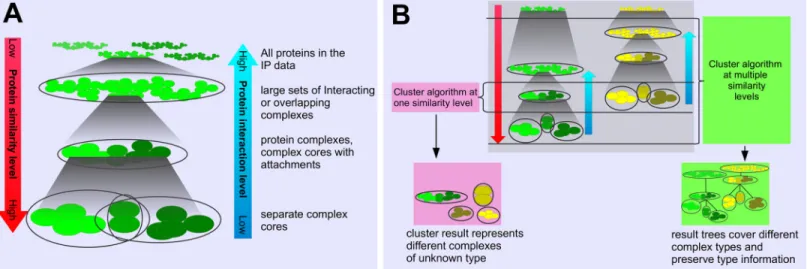
In the context of IP/MS data, proteins are considered“similar to each other”when they occur together across experiments and have similar abundance values. This often holds for pro-teins that build a complex together; however, the different characteristics of protein complexes lead to different similarity levels of their proteins in the data. This phenomenon is shown in Fig 1A. Firmly bound proteins within a complex core are very similar to each other because they occur together in similar abundance throughout large parts of the IP/MS data. A complex that consists of this core and different attachments appears as one set of proteins that are less similar than the core proteins. Interacting complexes can give rise to a single large set of pro-teins with relatively low similarity.
The similarity of interacting proteins in IP/MS data makes it possible to detect protein inter-action and complexes with clustering tools [3], which create clusters (sets of proteins) that rep-resent the complexes. Gavin et al. and Krogan et al. prep-resented large–scale IP/MS datasets from yeast and introduced methods to detect pairwise protein–protein interactions in their datasets [11–13]. Their datasets have been widely used for comparing further methods that find pro-tein–protein interactions or protein complexes [14–20], but there is no consensus on which method works best, and most publications do not distinguish between the different complex types. Malovannaya et al. showed in their large scale human IP study that protein complex cores can be found using an intuitive method that is based on searching for protein sets with high co-occurrence and reciprocal similarity [21,22]. The ideas from these publications were generalized in Kutzera et al. [23] and it was shown that the method works on datasets of differ-ent size and structure.
Different protein complexes at a specific interaction level, such as complex cores, do not always appear at the same similarity level in IP/MS data (Fig 1B). Most complex detection tools analyze the data at a specific (and often unknown) similarity level, and thus, their clusters may represent different types of complexes. To our knowledge, there is no clustering method that provides information about the interaction level or the similarity level of the found complexes. This complicates tuning the parameters of such methods to find a specific complex type and furthermore, hampers the interpretation of the results considerably.
the complexes. Moreover, unlike classical hierarchical clustering, HC4N allows for cluster over-lap at each level of the hierarchy.
Like previous methods, HC4N assigns proteins that are similar to each other to clusters. In addition, our method provides information about why proteins were clustered together and where these clusters can be split into smaller clusters of more similar proteins that represent complexes at a lower interaction level. This divide-and-conquer strategy makes it possible to capture different interaction levels from large sets of complexes down to the stable cores each complex is built of. New graphical result representation methods are part of HC4N. They visu-alize at which similarity level complexes are found in the data and make predictions about their interaction level possible. They also help in adjusting the method’s parameters to fit dif-ferent IP/MS datasets and finding difdif-ferent types of complexes.
Materials and Methods
Datasets
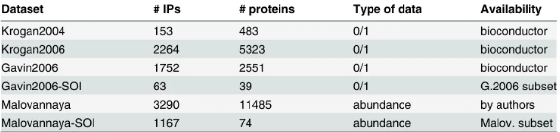
Several IP/MS datasets from yeast and humans are used to study the properties of our method and for comparison with other methods. Together with the IP/MS data, species–specific refer-ence protein complexes are needed for the evaluation.Table 1gives an overview of all IP/MS datasets and their types.
We used the large–scale yeast IP/MS dataset that was presented by Gavin et al. [11] and two IP/MS datasets from Krogan et al. [12,13]. We refer to these datasets as“Gavin2006,” “ Kro-gan2004”and“Krogan2006.”A subset from Gavin2006 (called“Gavin2006-SOI”) is created using HC4N (see the detailed analysis in the results section). As a complex reference for the yeast datasets, we used the well-established cyc2008 [7] catalog. This database contains an up– to–date reference set of 400 annotated yeast protein complexes and was previously used in other publications to evaluate complex prediction methods [17–19].
Fig 1. A: Proteins interact at different levels, from the low level of stable complex cores to the high level of temporarily interacting complexes. The different interaction types lead to different protein similarity levels in the context of the IP/MS data. Proteins of complex cores have a high similarity, while proteins of higher interaction levels have a lower similarity to each other.B: Two independent protein assemblies (depicted as green and yellow) and how they split in lower interaction levels. Protein complexes at different interaction levels can have the same similarity level. The clusters from a clustering method at one level (left) can represent complexes of different types for this reason, and it is unclear what each cluster represents. Our strategy (right) captures complexes at different similarity levels for this reason and creates trees that allow for predicting the interaction level.
The human IP/MS dataset of Malovannaya et al. [22] is the largest dataset in our analysis, and we refer to it as“Malovannaya.”From this dataset, we also derived a subset of certain pro-teins for which very precise information about complex–complex interactions is available. These proteins belong to the interaction complexes of“Mediator”(MED, [24]),“Integrator” (INT, [25]) and“RNA-Polymerase”(POL), which are described in two Malovannaya publica-tions [21,22]. We created an IP/MS subset (”Malovannaya-SOI”) that contains all these pro-teins and all corresponding IPs.
A satisfying reference for human protein complexes is still difficult to obtain. The best– known database for human interactions is CORUM [26]. However, complexes from CORUM are mainly functionally annotated, and unlike the complexes in cyc2008, they overlap highly due to redundancy in existing annotations [27]. Therefore, not every complex configuration from CORUM appears in the IP/MS data, which makes it difficult to use the database as a pro-tein complex reference. For the Malovannaya dataset, we used several sets of complexes from the Malovannaya publications as reference for this reason. A detailed list can be found inS1 Table. Information about the complex–complex interactions were obtained from the same publications.
The HC4N method
HC4N is based on the 4N method [23], which we will explain briefly here and in detail inS1 Text. 4N finds clusters called“near neighbor networks”in the IP/MS data. They are sets of sim-ilar proteins in terms of high pairwise co-occurrence, high set–wise completeness (all proteins in a near neighbor network co-occur highly with each other) and similar abundance. Each pro-tein is assigned to many near neighbor networks by the 4N method.
Three global threshold parameters, one for each of the three above–mentioned similarity types, are used to set the strictness for calculating the near neighbor networks. The co-occur-rence threshold parameter denotes in how many IPs two proteins need to co-occur relative to the number of IPs where any of them occur. The set–wise completeness parameter denotes how exclusive a near neighbor network needs to be. A low threshold allows for overlapping near neighbor networks, while a high threshold produces near neighbor networks that occur exclusively in this configuration. The abundance similarity is defined by the cosine similarity between two proteins.
The 4N method can set the thresholds for co-occurrence and set–wise completeness auto-matically to the strictest setting at which no proteins are lost, and it also returns the values as user feedback. The abundance similarity parameter is of minor importance (and not applicable for 0/1 data) and set by hand to 40 in all experiments. At low strictness settings, proteins with at least low similarity are assigned to large clusters that then represent a high protein interac-tion level. Proteins with high similarity are assigned to clusters when 4N is applied with high Table 1. IP/MS datasets used for the analyses.
Dataset # IPs # proteins Type of data Availability
Krogan2004 153 483 0/1 bioconductor
Krogan2006 2264 5323 0/1 bioconductor
Gavin2006 1752 2551 0/1 bioconductor
Gavin2006-SOI 63 39 0/1 G.2006 subset
Malovannaya 3290 11485 abundance by authors
Malovannaya-SOI 1167 74 abundance Malov. subset
strictness settings, and they represent a low interaction level. Clusters that overlap by a certain percentage (usually 50%) are joined to larger clusters, creating the final result of 4N.
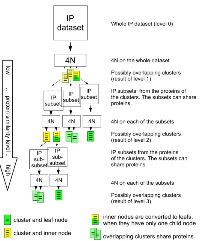
The HC4N strategy uses the ability of 4N to capture clusters at different similarity levels. It starts by applying 4N with low strictness to the IP/MS dataset. The resulting clusters are at level 1 in the result hierarchy tree; seeFig 2. They represent remotely interacting proteins at a high interaction level. For each of the (possibly overlapping) protein clusters, HC4N creates an IP/MS subset of its proteins by extracting the proteins and all IP experiments where they occur. Next, these subsets are analyzed using 4N with higher strictness. This second set of clusters represents level two in the result tree: a higher protein similarity level and a lower protein interaction level. The clusters are used again to create smaller IP/MS subsets, and again, they are analyzed with a stricter setup of 4N. This continues until the clusters cannot be split further.
The parameters of HC4N are set manually for the first level (see the result section for details). A manual setting of the parameters for all levels would be impossible as the total num-ber of parameters can get very large. Therefore, the parameters for the higher levels are set automatically to the highest values where all proteins from the current subset are assigned to at least one cluster. As each subset is divided into smaller subsets of more similar proteins in a step, the HC4N strategy automatically captures a higher protein similarity level than before. Clusters of one step can have proteins in common. This facilitates, for example, that a core with different attachments can appear as a different cluster for each combination of core and attachments.
The result of HC4N is a tree–structured graph where the root node (level 0) contains all proteins in the IP/MS dataset. The root node has a child node for each level–1 cluster. Each node contains a cluster that is calculated from the subset of the previous node in the hierar-chy. A node is a leaf when its cluster is not split further or an inner node with child nodes when its cluster is split into smaller clusters. The protein similarity of each cluster is judged using the minimum co-occurrence of its proteins. A cluster with a low co-occurrence repre-sents proteins with low similarity at a high interaction level. Clusters with a high occur-rence represent a low interaction level. Child nodes of an inner node have a higher co-occurrence than their parent node, as they were built by splitting the parent node into pro-teins of higher similarity.
Visualization of the HC4N result is crucial for interpreting the results and can be done in different ways. One way is the“hierarchical cluster plot”(HC-plot, seeFig 3), a heatmap–type diagram showing all proteins vs. each other. The HC-plot visualizes clusters at different co-occurrence levels. It shows which proteins are in a cluster together with a certain co-co-occurrence and whether this cluster is split into smaller clusters of higher co-occurrence. A cluster at a low protein similarity level occurs as a large square with a deep blue color in the HC plot. When the cluster has child clusters at a higher similarity level, they appear within that square as brighter colored, smaller squares. The plot also shows at which similarity level the clusters cannot be split further. Details about creating the HC-plot can be found inS1 Text. The HC-plot does not visualize every detail of the HC4N result; however, it gives insight into the different similarity levels, especially for large datasets, which are hard to visualize. It also helps in selecting the strictness for the first level of HC4N.
Fig 2. General overview of the HC4N strategy.The IP/MS dataset is analyzed with 4N to create the clusters of level 1. The dataset is split up into subsets where each subset contains all proteins from a level–1 cluster. 4N is applied to each of the subsets to create level 2. The procedure is repeated to create levels 3 and above, until no further splits are possible.
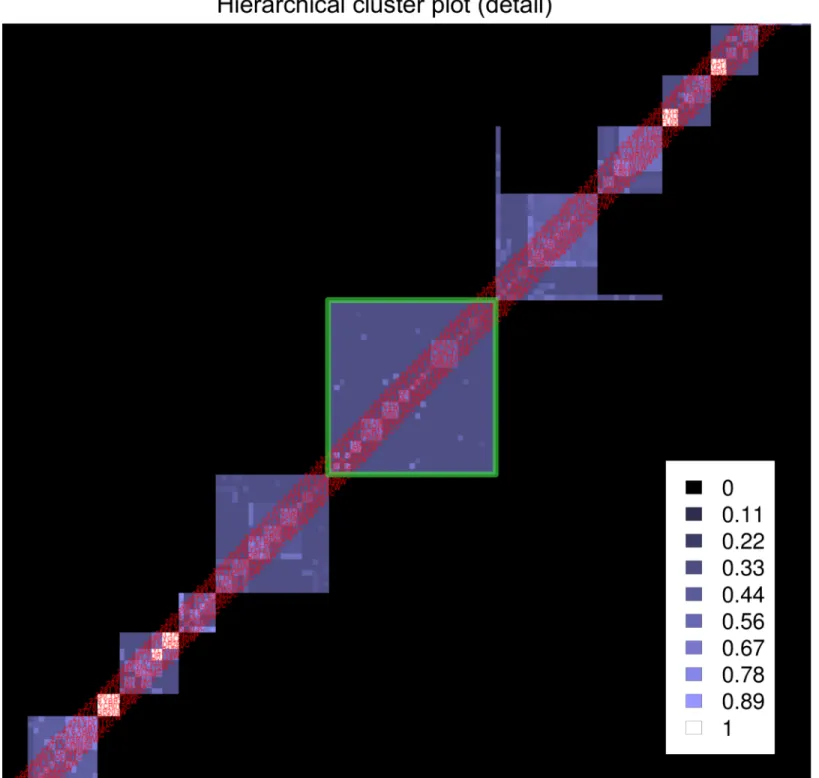
Clusters with a low co-occurrence and with many child clusters of higher co-occurrence represent sets of overlapping or interacting protein complexes and should receive special atten-tion. We call such clusters subsets of interest (SOIs). They appear in the HC-plot as large squares with complex inner structures as shown inFig 5. HC4N, with parameters optimized for the large–scale dataset, might not reveal the correct inner composition of each SOI. For this reason, the dataset derived from a SOI should be treated as a new (small) dataset and analyzed again with HC4N.
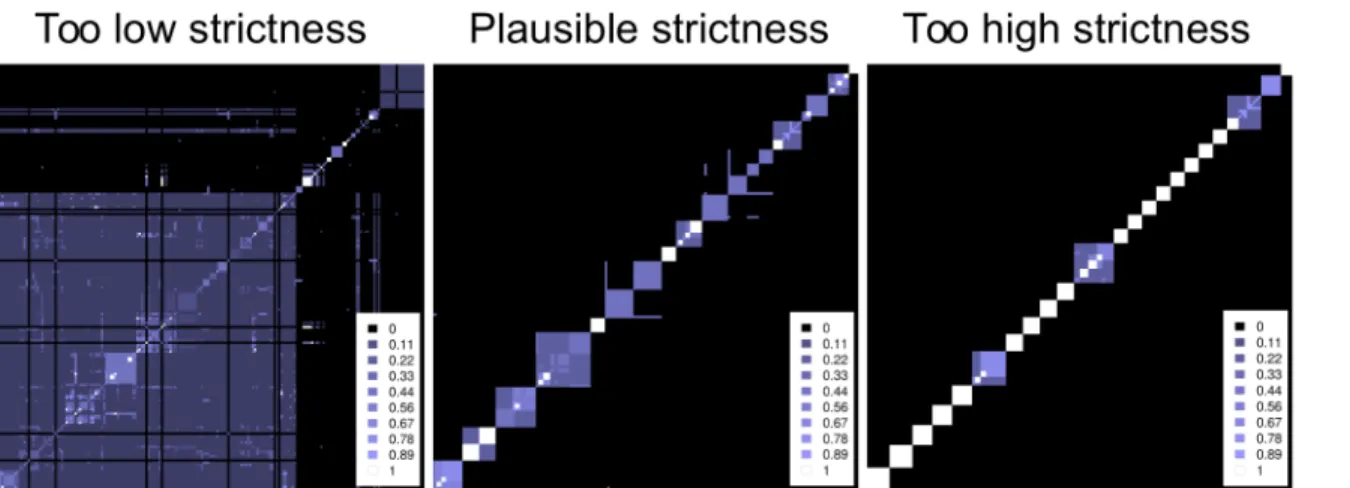
Fig 3. Example hierarchical cluster plots for different co-occurrence thresholds at HC4N level 1.The plots are small cutouts from the analysis of the Krogan2004 dataset. Left: The threshold is set too low with 0.125. Randomly co-occurring proteins lead to large, highly overlapping clusters, which do not represent protein complexes. At a higher threshold of 0.35, the clusters overlap less, and possible complexes and cores are visible. At a too–high threshold of 0.6, the clusters represent mostly complex cores, and their relation to each other is not visible. HC4N sets the set–wise completeness threshold automatically to 0.64 in all three examples.
doi:10.1371/journal.pone.0139704.g003
Fig 4. Example HC4N result tree.For clarity, the co-occurrence is displayed in each node. Clusters with many proteins of low co-occurrence and with large child nodes indicate interacting complexes at the highest interaction level. Complexes built of several cores have a higher co-occurrence and leafs as child nodes. Leaf nodes with a high co-occurrence symbolize complex cores. Leaf nodes with low co-occurrence mostly do not represent complex cores, and their interpretation is not always univocal.
Fig 5. Extract from the HC–plot of Gavin2006 showing subsets of interest (SOIs).The green square frames the SOI of the three POL complexes. Black represents that two proteins are never in the same cluster, dark blue colors represent clusters with a low co-occurrence and bright colors represent clusters with a high co-occurrence.
Other IP/MS analysis methods
SOIs are small, which makes it possible to analyze them with other methods for which the full dataset would be too large. We will discuss the SOI analysis with the methods Biclust [29], HICLAS [30] and apComplex [31] in this publication. Biclust [29] is used for inducing highly overlapping protein complexes from dense small–scale IP/MS datasets. The method is probabi-listic, and as it needs many iterations to give reliable results, it is very computationally inten-sive. Biclust can process both occurrence and abundance data.
The HICLAS (HIerarchical CLASses analysis) [30,32] algorithm has not yet been used for IP/MS analysis, but its underlying model fits the expected effects of overlapping clusters on pure 0/1 data and it was tested for that reason. An HICLAS model withKclusters createsK protein clusters andKIP clusters. In the model, anI×Jprotein by IP datasetDis approxi-mated by a model matrixMof the same size.Mis composed asM=AB, whereAis aI×K binary matrix withAi,kdenoting whether proteiniis in protein clusterk,Bis aJ×Kbinary
matrix withBj,kdenoting whether IPjis in IP clusterkandis a binary matrix multiplication operator where each result>0 is set to 1, for example, 1+1 = 1. HICLAS minimizes the residu-als functionfover the matricesAandB, wherefdenotes the sum of squared differences between the model matrixMand data matrixDas
fðA;BÞ ¼XI i¼1
XJ
j¼1
ðDi;jMi;jÞ2: ð1Þ
We applied HICLAS in our tests with different numbers of clusters and examined the resid-uals of each analysis to find the optimal number of clusters. We used the possibility to weight negative residuals differently than positive residuals [33].
The method apComplex [14,31] uses a local modeling algorithm on the bait-prey interac-tion graph to reconstruct possible complexes in pure occurrence data and was previously used for analyzing the yeast datasets.
Cluster quality assessment
The tree–shaped graphs from our HC4N method contain more information than just the clus-ters themselves; however, no comparison method that takes this additional information into account is available. To make the comparison possible, we removed the tree information from the result and joined clusters that were overlapping by more than 60%. The same joining step was applied to the results of the other methods for a fairer comparison. This joining step increased the quality of all methods because they often produce numerous, very similar small clusters that, when joined, represent the reference complexes better.
We used the method by Brohée and van Helden [34] to evaluate our results. The method is capable of measuring how accurately a set of reference complexes is predicted by a set of clus-ters, and it has already been used to assess complex predictions in other studies [17,18]. Three quality measures are provided by the method: sensitivity, positive predictive value (PPV) and accuracy. The sensitivity is the fraction of proteins from the reference complexes that are found in the predicted clusters; the PPV is the fraction of proteins from the predicted clusters that belong to the reference complexes. From sensitivity and PPV, the accuracy is calculated as the square root of their product. For a set of predicted clusters and a reference complex set, an accuracy of 1 is reached when each reference complex perfectly matches one of the clusters.
called separation is provided by the method in addition, denoting how many predicted com-plexes represent one reference complex. The separation score is 1 when each predicted complex covers exactly one reference complex.
In our comparison, not all analysis methods could be applied to all datasets. For apComplex, the large datasets do not produce results due to memory problems when running on a PC with 12 gigabytes of memory. Both Biclust and HICLAS did not produce results on the large sets within a reasonable amount of time.
Results
The HC4N performance depends on optimal parameters for level 1. To find these parameters, we initially allowed HC4N to create the level–1 clusters with automatic setup where the thresh-olds for co-occurrence and set–wise completeness are set as high as possible so that each pro-tein is still assigned to at least one cluster.
We examined the HC-plot for the result to determine at which protein co-occurrence level the first clusters appear. When the clusters were too large, we set the co-occurrence threshold slightly higher than before, and when they were overlapping too much, we set the complete-ness parameter higher. For the SOI analyses, we have set the co-occurrence threshold and set-completeness parameter slightly lower than in the automatic setup to detect the interaction level of complex–complex interactions (see below). A scheme for how to use HC4N is located inS2 Textand details for each large–scale analysis, including Figures, are inS3 Text.
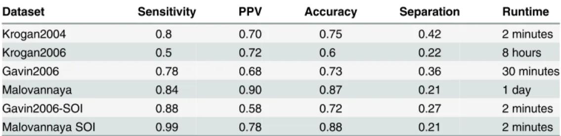
The results are summarized inTable 2. HC4N gains good sensitivity and PPV for most data-sets. The separation values are between 0.2 and 0.42, which is acceptable but shows that HC4N, like most methods, tends to create slightly too many clusters. A better separation value would be achieved by joining the clusters with a lower threshold at the cost of a lower specificity.
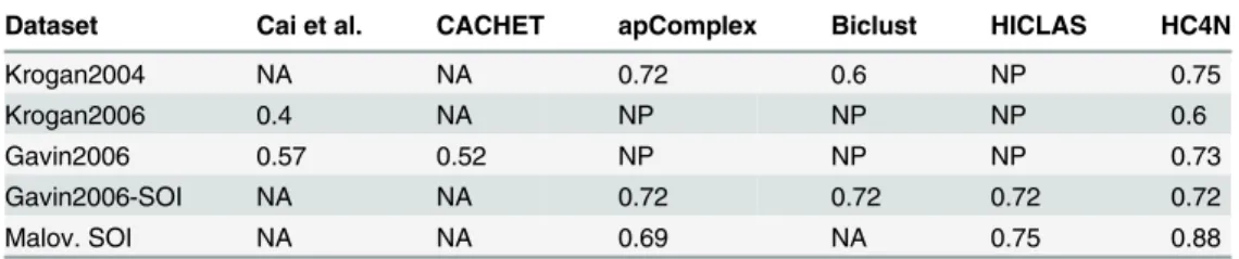
Table 3compares our accuracy with other methods. We obtained the scores for Biclust, HICLAS and apComplex by applying the methods ourselves; the results for Wu et al. [17] and Cai et al. [18] were taken from the original publications. The table shows that our method has better accuracy in most cases. The dataset Krogan2004 is of low complexity, and previous methods already gained an accuracy of 0.72, which was still increased to 0.75 by HC4N. A more substantial improvement was reached for Gavin2006 (0.73 compared to 0.57). Kro-gan2006 is difficult to analyze, which is why previous methods scored below 0.5 and also why HC4N only achieves 0.6.
When compared to other methods, HC4N does not always yield a larger separation score (seeS2 Table). In these cases, however, HC4N and the other methods give separation scores that are in the same range. The two SOIs deserve a more detailed analysis as they contain over-lapping and interacting complexes. They are discussed below.
Table 2. Summarized results of HC4N on all tested datasets.
Dataset Sensitivity PPV Accuracy Separation Runtime
Krogan2004 0.8 0.70 0.75 0.42 2 minutes
Krogan2006 0.5 0.72 0.6 0.22 8 hours
Gavin2006 0.78 0.68 0.73 0.36 30 minutes
Malovannaya 0.84 0.90 0.87 0.21 1 day
Gavin2006-SOI 0.88 0.58 0.72 0.27 2 minutes
Malovannaya SOI 0.99 0.78 0.88 0.21 2 minutes
Analysis of the Gavin2006-SOI dataset
The HC-plot from the Gavin2006 analysis shows subsets of interest, and we analyzed the green–framed SOI (seeFig 5) as an example. We assume for this demonstration that we do not know what type of complexes the cluster of the SOI contains. The subset Gavin2006-SOI con-tains all proteins from the cluster and all IPs in which any of the proteins occur.
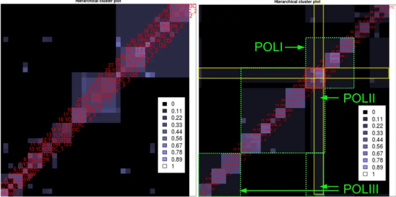
Analyzing the dataset starts by running HC4N with automatic setup and inspecting the HC-plot. The plot shows complexes but only a few connections between them, as shown in Fig 6, left side. We already know that all proteins have a certain degree of similarity because they were assigned to one cluster in the large–scale analysis. We conclude that the automatic parameters are too strict and not optimal for finding clusters with shared proteins. Therefore, the parameters are lowered until the new HC-plot (Fig 6, right) shows a characteristic pattern that denotes shared proteins. This pattern features proteins (which are the shared proteins) with a very high co-occurrence to each other and a high co-occurrence to many other proteins from different clusters. In the figure, the pattern contains YOR224C and YBR154C, which have a high co-occurrence to almost all proteins in the plot. Two other proteins (YOR210W, YPR187W) have a high co-occurrence to these two proteins. Three large clusters are shown in the HC-plot, and the two proteins appear in all of them. We can assume that the SOI contains (at least) three clusters that share the proteins from the pattern. The two other proteins that are similar to the shared proteins are likely to be shared as well.
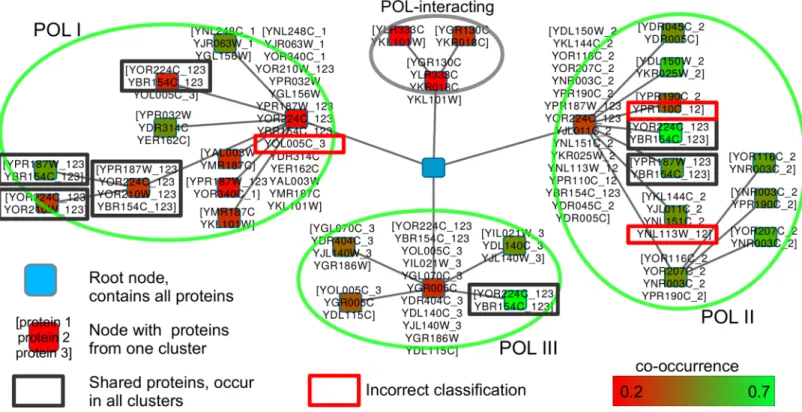
A comparison with the cyc2008 reference shows that the three clusters represent the three POL complexes and that the four mentioned proteins are shared by them. The cluster result does not show that two additional proteins are shared between POLI and POLII, as they are exclusively assigned to POLII. Twelve SOI proteins are not in the cyc2008 reference. They were searched on string-DB (www.string-db.org) [35], a graph–based on–line protein interaction database. We included the interaction types“Co-occurrence”and“Experiments”into the string-DB result, but no genetic information. We found that ten proteins interact with the POL complexes to which they were assigned by HC4N. A network from string-DB showing all POL proteins and the additional proteins can be found inS1 Fig.
The cytoscape visualization of the result graph (Fig 7) confirms the findings. It shows four clusters, of which the three largest clusters represent the three POL-complexes. The two pro-teins (YOR224C and YBR154C) appear in all clusters, and therefore we can assume that YOR224C and YBR154C interact with all complexes. The two proteins also appear together Table 3. Accuracy of HC4N in comparison to competing methods.
Dataset Cai et al. CACHET apComplex Biclust HICLAS HC4N
Krogan2004 NA NA 0.72 0.6 NP 0.75
Krogan2006 0.4 NA NP NP NP 0.6
Gavin2006 0.57 0.52 NP NP NP 0.73
Gavin2006-SOI NA NA 0.72 0.72 0.72 0.72
Malov. SOI NA NA 0.69 NA 0.75 0.88
The values for CACHET [17] and Cai et al. [18] were taken from the respective publications. We applied the other methods on all datasets.“NA”means that no value for this dataset was available in the corresponding original publication.“NP”means that we tried the method on the dataset but it was not possible to produce a result.
multiple times with YOR210W and YPR187W, which denotes that all four proteins play an important role in all three POL complexes.
The SOI was also analyzed with apComplex, BICLUST and HICLAS. ApComplex creates more than 200 clusters, leading to an accuracy of 0.76 but very poor separation of 0.05. After joining the clusters, a still–good accuracy of 0.72 at a now–good separation of 0.34 is reached. In all cases, apComplex misclassifies several proteins.
Too many and too–small clusters are built by BICLUST, which represent the POL com-plexes only partly and did not show the special role of the shared proteins. HICLAS was better able to capture POL but requires the cluster number as prior knowledge. None of the methods provides information about the interaction level of the clusters. A graphical comparison of the results between HC4N, BICLUST and HICLAS can be found inS4 Text.
Analysis of the Malovannaya-SOI dataset
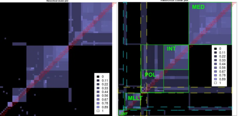
HC4N is applied with automatic settings, and the HC-plot is examined (Fig 8, left). Several clusters are visible but only a few connections between them. We know based on the protein selection that their clusters interact, and now we want to explore these interactions in detail. We set the strictness for level 1 low enough such that the HC-plot shows the characteristic pat-terns indicating complex interactions. The new plot (Fig 8, right) shows two large and two small clusters of different structure. While one large cluster is dense and with high co-Fig 6. Hierarchical cluster plots for two different HC4N parameter settings on the Gavin2006-SOI dataset.The numbers at the labels (_1,_2,_3,_12, _123) show the POL-cluster assignments according to cyc2008.Left: Too–strict parameter settings (co-occurrence threshold 0.25, completeness threshold 0.4): The clusters are scattered and show low overlap. It is not clear which proteins are shared by how many complexes.Right: Lower parameters (0.2 and 0.5). The green frames show the three POL complexes as the HC4N result. The red square shows a characteristic pattern of four highly co-occurring proteins that in addition, partly co-occur with most other proteins (yellow frames). They are the shared proteins of the three complexes.
occurrence, the other has a lower co-occurrence and two dense subclusters of more similar pro-teins are visible within it. Two of the characteristic patterns, one with two and one with four proteins, occur across several but not all clusters.
We conclude from the plot that the large cluster of lower co-occurrence is built from two closely interacting subcomplexes, one containing the proteins of the four-protein pattern that facilitates the interaction between the two subcomplexes. One subcomplex also interacts sepa-rately with the large dense complex but less closely. The two-protein pattern indicates interac-tion of the large dense complex with the two other small complexes.
The comparison with the reference shows that the MED complex is represented by the large dense cluster and that the complexes POL and INT are the two subcomplexes of the other clus-ter. The proteins POLR2A/B/C/G build the four-protein pattern, and it is known that they facilitate the interaction between POL and INT as well as between POL and MED. It is also known that POL and INT build a complex together, while POL and MED interact more tran-siently. The two-protein pattern includes ELL and SPEN, which connect the small complex around MLLT and ZNF to MED but not to INT.
All conclusions agree with the information from [22] and [36]. We also created the network representation, seeS5 Text. It allows the same conclusions and shows in a clearer manner which protein interaction level is represented by which similarity level. MED and INT are indi-vidually assigned to POL (but not to each other) in higher interaction levels, and the complexes separate in the lower levels. The same holds for the small complexes that interact with MED. In Fig 7. Network representation of the Gavin2006-SOI HC4N result.The green ovals indicate the three POL complexes as found by HC4N. The forth oval (gray) contains proteins that are known to interact with POL but were not in the cyc2008 reference. The protein name suffixes (_1,_2,_3,_12,_123) indicate the assignment to POLI-POLIII from the reference. The four shared proteins from the characteristic pattern (framed in dark gray) occur in all complexes and together multiple times.
this specific dataset, the protein co-occurrence is relatively low, even within POL, MED and INT, but still higher relative to the complex–complex interaction forms POLR-MED and POL-INT.
The dataset was also analyzed with apComplex and HICLAS (seeS4 Text). We were not able to run Biclust because the dataset is too large. As with the other SOI analysis, the methods were not able to capture the complexes correctly and created too many too–small clusters. None of the methods is designed to uncover the different levels of interaction between the com-plexes, and from their results, it is not clear which interaction level their clusters represent.
Discussion and Conclusions
Finding protein complexes in IP/MS data is a difficult task. Protein complexes can be found at different organizational levels in IP/MS data, and these levels must be explored together. The task is twofold: i) finding the complexes at different levels and ii) visualizing the result in a way that makes the different levels visible. In essence, this is a data exploration and visualization problem, and we designed our method, HC4N, to address that problem.
Exploratory data analysis is a partly subjective task, e.g., by selecting parameters during analysis. While most software tools come with default parameters, understanding their effect on the result remains a problem. Our method not only supports automatic and manual param-eter settings but also allows the user to retrace the effect of paramparam-eter changes with visual Fig 8. Hierarchical cluster plots for the Malovannaya SOI. Left: With too–strict automatic thresholds (co-occurrence 0.09, completeness 0.6), correct clusters are visible but not the connections between them.Right: Lower parameters (0.05 and 0.5) create patterns indicating shared proteins. Two large and two small clusters are visible, framed by the thick green squares. MED appears as a separate cluster, while INT and POL appear together as dense subsets of one cluster. POL and INT can build a more stable complex together than POL and MED. One pattern (framed in yellow) contains POLR2 A/B/C/G, which are important interactors within both the POL-INT and the POL-MED complex. ELL2 and SPEN (framed in cyan) comprise another pattern and are important for the interaction between MLLT and the MED complex.
feedback. The change of parameters is very insightful because it enables exploring the different levels of organization of the protein complexes in a given dataset.
A major problem for all complex finding tools is noise in the IP/MS data, leading to many false positives. While HC4N cannot actively remove noise, its built–in visualization tools help in detecting noise. In noisy data, HC4N will find many small, possibly false-positive clusters at low co-occurrence levels when applied with automatic parameters. Detected true-positive clus-ters may not have a fundamentally higher co-occurrence than the false positives. This leads to characteristic HC-plots without the typical clusters of high co-occurrence that appear when analyzing low-noise datasets. The behavior is demonstrated with examples inS3 Text.
We have shown in this manuscript that protein complexes occur at different interaction and similarity levels, even in the same IP/MS dataset. Our new method, HC4N, is able to find com-plexes of different types and has been validated thoroughly using several datasets and compari-sons with existing methods. The philosophy behind HC4N is to provide an interactive
exploratory tool for analyzing IP/MS data that can be used (and tuned) by the biologists.
Supporting Information
S1 Table. Reference complexes for the Malovannaya datasets.Reference from Malovannaya et al..
(PDF)
S2 Table. HC4N separation scores.Separation scores of HC4N in comparison with the other methods.
(PDF)
S1 Text. 4N, HC4N, HC-plot, pseudocode.Details for 4N, HC4N and the hierarchical cluster plot. pseudocode for all modules.
(PDF)
S2 Text. General HC4N strategy.Usage and parameter selection strategy for HC4N. (PDF)
S3 Text. HC4N analyses.HC4N analyses on the large–scale datasets. (PDF)
S4 Text. Biclust, apComplex, HICLAS.Analysis of Gavin2006-SOI and Malovannaya-SOI with Biclust, apComplex, HICLAS.
(PDF)
S5 Text. Malovannaya-SOI HC4N graph.HC4N result graph for the Malovannaya-SOI anal-ysis.
(PDF)
S1 Fig. POL StringDB.All proteins of the Gavin2006-SOI dataset as string-DB network. (TIFF)
Acknowledgments
Author Contributions
Conceived and designed the experiments: JK HCJH AKS TFW. Performed the experiments: JK. Analyzed the data: JK. Contributed reagents/materials/analysis tools: JK. Wrote the paper: JK HCJH AKS.
References
1. Alberts B. The cell as a collection overview of protein machines: Preparing the next generation of molecular biologists. Cell. 1998; 92:291–294. doi:10.1016/S0092-8674(00)80922-8PMID:9476889
2. Alberts B, Johnson A, Lewis J, Raff M, Roberts Kea. Molecular Biology of the Cell 5E. 5th ed. Garland Science; 2008.
3. Gavin AC, Bösche M, Krause R, Grandi P, et al M. Functional organization of the yeast proteome by systematic analysis of protein complexes. Nature. 2002; 415(6868):141–147. doi:10.1038/415141a PMID:11805826
4. Clancy T, Andreas E, Nygard Sl, Hovig E. Predicting Physical Interactions between Protein Complexes. Mol Cell Proteomics. 2013; 12(6):1723–34. doi:10.1074/mcp.O112.019828PMID:23438732
5. Pizzuti C, Rombo SE. Algorithms and tools for protein-protein interaction networks clustering, with a special focus on population-based stochastic methods. Bioinformatics. 2014; 30(2000):1–9.
6. Clancy T, Hovig E. From proteomes to complexomes in the era of systems biology. Proteomics. 2014 Jan; 14(1):24–41. doi:10.1002/pmic.201300230PMID:24243660
7. Pu Shuye and Wong Jessica and Turner Brian and Cho Emerson and Wodak Shoshana J. Up-to-date catalogues of yeast protein complexes. Nucleic acids research. 2009 Feb; 37(3):825–31. doi:10.1093/ nar/gkn1005PMID:19095691
8. Drewes G, Bouwmeester T. Global approaches to protein–protein interactions. Current opinion in cell biology. 2003; 15(2):199–205. doi:10.1016/S0955-0674(03)00005-XPMID:12648676
9. Gentleman R, Huber Wea. Making the most of high-throughput protein-interaction data. Genome Biol. 2007; 8(10):112. doi:10.1186/gb-2007-8-10-112PMID:18001486
10. Bensimon A, Heck AJR, Aebersold R. Mass spectrometry-based proteomics and network biology. Annual review of biochemistry. 2012; 81:379–405. doi:10.1146/annurev-biochem-072909-100424 PMID:22439968
11. Gavin AC, Aloy P, Grandi P, Krause R, Boesche Mea. Proteome survey reveals modularity of the yeast cell machinery. Nature. 2006; 440(7084):631–6. doi:10.1038/nature04532PMID:16429126
12. Krogan NJ, Peng WT, Cagney G, Robinson MD, Haw Rea. High-definition macromolecular composi-tion of yeast RNA-processing complexes. Molecular cell. 2004; 13(2):225–39. doi: 10.1016/S1097-2765(04)00003-6PMID:14759368
13. Krogan NJ, Cagney G, Yu H, Zhong G, Guo Xea. Global landscape of protein complexes in the yeast Saccharomyces cerevisiae. Nature. 2006; 440(7084):637–643. doi:10.1038/nature04670PMID: 16554755
14. Scholtens D, Gentleman R. Making sense of high-throughput protein-protein interaction data. Statistical applications in genetics and molecular biology. 2004 Jan; 3(1):Article39. PMID:16646819
15. Kim EDH, Sabharwal A, Vetta AR, Blanchette Mea. Predicting direct protein interactions from affinity purification mass spectrometry data. Algorithms for Molecular Biology. 2010; 5(1):34. doi:10.1186/ 1748-7188-5-34PMID:21034440
16. Geva G, Sharan R. Identification of protein complexes from co-immunoprecipitation data. Bioinformat-ics. 2011 Jan; 27(1):111–7. doi:10.1093/bioinformatics/btq652PMID:21115439
17. Wu M, Li XL, Kwoh CK, Ng SK, Wong L. Discovery of Protein Complexes with Core-Attachment Struc-tures from Tandem Affinity Purification (TAP) Data. Journal of computational biology. 2011 Jul; 18 (0):1–16.
18. Cai B, Wang H, Zheng H, Wang H. Detection of protein complexes from affinity purification/mass spec-trometry data. BMC systems biology. 2012 jan; 6, Suppl 3(S4).
19. Xie Z, Kwoh CK, Li XL, Wu M. Construction of co-complex score matrix for protein complex prediction from AP-MS data. Bioinformatics. 2011; 27(13):i159–i166. doi:10.1093/bioinformatics/btr212PMID: 21685066
21. Malovannaya A, Li Y, Bulynko Y, Jung SY, Wang Yea. Streamlined analysis schema for high-through-put identification of endogenous protein complexes. Proceedings of the National Academy of Sciences. 2010; 107(6):2431–2436. doi:10.1073/pnas.0912599106
22. Malovannaya A, Lanz RB, Jung SY, Bulynko Y, Le NTea. Analysis of the human endogenous coregula-tor complexome. Cell. 2011; 145(5):787–799. doi:10.1016/j.cell.2011.05.006PMID:21620140
23. Kutzera J, Hoefsloot HCJ, Malovannaya A, Smit AB, Mechelen IVea. Inferring protein-protein interac-tion complexes from immunoprecipitainterac-tion data. BMC research notes. 2013 Jan; 6:468. doi:10.1186/ 1756-0500-6-468PMID:24237943
24. Taatjes DJ. The human Mediator complex: a versatile, genome-wide regulator of transcription. Trends in biochemical sciences. 2010; 35(6):315–322. doi:10.1016/j.tibs.2010.02.004PMID:20299225
25. Baillat D, Hakimi MA, Näär AM, Shilatifard A, Cooch Nea. Integrator, a multiprotein mediator of small nuclear RNA processing, associates with the C-terminal repeat of RNA polymerase II. Cell. 2005; 123 (2):265–276. doi:10.1016/j.cell.2005.08.019PMID:16239144
26. Ruepp A, Waegele B, Lechner M, Brauner B, et al DK. CORUM: the comprehensive resource of mam-malian protein complexes–2009. Nucleic acids research. 2010 Jan; 38(Database issue):D497–501. doi:10.1093/nar/gkp914PMID:19884131
27. Havugimana PC, Hart GT, Nepusz T, Yang H, Turinsky ALea. A census of human soluble protein com-plexes. Cell. 2012 Aug; 150(5):1068–81. doi:10.1016/j.cell.2012.08.011PMID:22939629
28. Smoot ME, Ono K, Ruscheinski J, Wang PL, Ideker T. Cytoscape 2.8: new features for data integration and network visualization. Bioinformatics (Oxford, England). 2011 Feb; 27(3):431–432. doi:10.1093/ bioinformatics/btq675
29. Choi H, Kim S, Gingras AC, Nesvizhskii AI. Analysis of protein complexes through model-based biclus-tering of label-free quantitative AP-MS data. Molecular systems biology. 2010; 6(1). doi:10.1038/msb. 2010.41PMID:20571534
30. Wilderjans TF, Ceulemans E, Van Mechelen I. The SIMCLAS model: Simultaneous analysis of coupled binary data matrices with noise heterogeneity between and within data blocks. Psychometrica. 2012; 77:724–740. doi:10.1007/s11336-012-9275-3
31. Scholtens D, Vidal M, Gentleman R. Local modeling of global interactome networks. Bioinformatics (Oxford, England). 2005 Sep; 21(17):3548–57. doi:10.1093/bioinformatics/bti567
32. De Boeck P, Rosenberg S. Hierarchical classes: Model and data analysis. Psychometrica. 1988; 53:361–381. doi:10.1007/BF02294218
33. Leenen I, Van Mechelen I, Gelman A, De Knop S. Bayesian hierarchical classes analysis. Psychome-trica. 2008; 73:39–64. doi:10.1007/s11336-007-9038-8
34. Brohée S, van Helden J. Evaluation of clustering algorithms for protein-protein interaction networks. BMC bioinformatics. 2006; 7:488. doi:10.1186/1471-2105-7-488PMID:17087821
35. Szklarczyk D, Franceschini A, Kuhn M, Simonovic M, Roth Aea. The STRING database in 2011: func-tional interaction networks of proteins, globally integrated and scored. Nucleic acids research. 2011; 39 (suppl 1):D561–D568. doi:10.1093/nar/gkq973PMID:21045058