5286.pdf

(1)

Interactive Sound Propagation using

Precomputation and Statistical Approximations

Lakulish Antani

A dissertation submitted to the faculty of the University of North Carolina at Chapel Hill in partial fulfillment of the requirements for the degree of Doctor of Philosophy in the Department of Computer Science.

Chapel Hill 2013

(2)

ABSTRACT

LAKULISH ANTANI: Interactive Sound Propagation Using Precomputation and Statistical Approximations

(Under the guidance of Dinesh Manocha.)

(3)

(4)

(5)

Acknowledgments

The past five years spent working in the Department of Computer Science at UNC Chapel Hill on the research that ultimately formed this dissertation have been mem-orable. I would like to thank the many people who played an important role in my journey and professional evolution. First of all, I would like to thank my advisor, Prof. Dinesh Manocha, for his guidance and support, as well as the freedom I was provided throughout the course of this work. I would also like to thank the members of my committee, Prof. Gary Bishop, Prof. Ming C. Lin, Prof. Anselmo Lastra, and Dr. Nikunj Raghuvanshi, for their insightful feedback and discussions on my research work and this dissertation.

I would also like to thank the many talented collaborators I have had the privilege of working with, including Anish Chandak, Micah Taylor, Ravish Mehra, Sean Cur-tis, Hengchin Yeh, and Zhimin Ren. I would also like to thank Prof. Lauri Savioja and Dr. Tapio Lokki at Aalto University, and Adam Lake at Intel Corporation for their collaboration and insight. I would also like to thank the many anonymous reviewers who have helped me improve the quality of my work.

(6)

WR91CRB-08-C-0137.

(7)

List of Tables

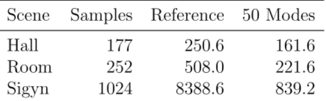
4.1 Performance of direct-to-indirect transfer for diffuse reflections. . . 57

4.2 Memory required by diffuse transfer operators. . . 58

4.3 Comparison of direct-to-indirect transfer with ART. . . 59

5.1 Performance and memory overhead of precomputing compact acoustic transfer operators. . . 74

5.2 Run-time performance of compact acoustic transfer operators. . . 74

6.1 Performance of local distance average estimation. . . 87

7.1 Performance of proxy-based higher-order reflections. . . 96

(13)

List of Figures

1.1 Examples of video games . . . 3

4.1 Overview of direct-to-indirect diffuse transfer. . . 52

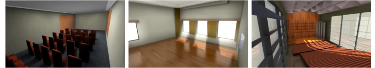
4.2 Benchmark scenes for direct-to-indirect diffuse transfer. . . 57

4.3 Diffuse IRs computed with and without SVD compression. . . 60

4.4 SVD approximation error for diffuse transfer operators. . . 60

4.5 SVD approximation error with increasing reflection orders. . . 61

5.1 Overview of sound propagation with compact acoustic transfer oper-ators. . . 63

5.2 Dynamic source shadowing. . . 71

5.3 Benchmark scenes for compact acoustic transfer operators. . . 72

5.4 SVD truncation error during KLT basis construction. . . 75

5.5 Energy decay curves computed with compact acoustic transfer operators. 77 6.1 Spatial and directional variation of mean free path. . . 82

6.2 Sampling directions to compute local distance average. . . 83

6.3 Benchmark scenes for ambient reverberance and aural proxies. . . 87

6.4 Convergence of local distance average estimate. . . 88

6.5 Accuracy of representing local distance with spherical harmonics. . . 88

7.1 Higher-order reflections using a rectangular aural proxy. . . 92

7.2 Convergence of proxy size estimation. . . 97

(14)

Chapter 1 Introduction

Computer graphics has made significant progress in the last few decades. Video games, film, and animation have driven the development of improved graphics tech-niques and hardware, as well as popularized their use, to the point that computer graphics is now a household name. In addition to entertainment applications, com-puter graphics has helped revolutionize the ways in which we interact with comput-ers (through rich graphical user interfaces) and the ways in which we interpret data (through, for example, scientific or medical visualization). In fact, computer graphics techniques such as graphics processing units (GPUs) have made a profound impact on fields as diverse as oil exploration and finance.

(15)

of virtual environments. However, this process typically involves manual recording of real-world sounds, or manual tuning of acoustic filters [33]. Acoustic simulation or sound rendering techniques are rarely used in interactive applications due to their compute-intensive nature.

The simulation of sound propagation, i.e., how sound waves behave in an envi-ronment, can be used to add realistic acoustic effects to interactive applications. To simulate sound propagation, we begin with the position of the sound source and the sound waves it emits. This is combined with a description of the 3D environment to simulate sound waves as they travel through the environment until they reach a listener position. This thesis presents techniques for performing sound propagation in interactive applications, to add acoustic effects in real-time.

1.1 Applications

There are a wide range of applications that can benefit from improved (i.e., more accurate, more efficient, or both) sound propagation simulation. Some of these ap-plications are briefly summarized below, along with the manner in which they use (or may use) sound propagation simulation.

1.1.1 Games

(16)

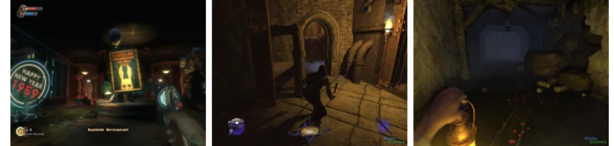
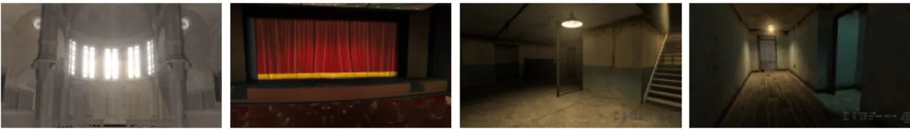
Figure 1.1: Examples of video games with gameplay that stands to benefit from sound propagation effects. Left: Bioshock [1], a first-person shooter. Sound propagation can help players locate unseen enemies, even from behind cover. Center: Thief 3 [21], a stealth game. Sound propagation can help players track and evade enemies. Right: Amnesia [26], a survival horror game. Sound propagation can improve player immersion and heighten the emotional experience.

player immersion.

Another vital means of improving player immersion is through realistic audio ren-dering (or sound renren-dering). A wide variety of games benefit from the use of improved acoustic effects. In first-person shooter games such as Bioshock [1] (Figure 1.1), ene-mies (including hard-to-spot snipers) may attack the player from multiple directions, and are often located behind cover. In such situations, directional acoustic cues can often help players locate the enemies more quickly, leading to less frustrating game-play. In stealth-based games such as Thief [21] (Figure 1.1), the player must often evade wandering enemies, or track them without being seen. In such situations, too, acoustic cues (particularly those pertaining to reflected or occluded sound) can help players keep track of the whereabouts of enemies without having to maintain a line of sight. In survival horror games such asAmnesia [26] (Figure 1.1), improved acoustic effects can significantly improve immersion, and the level of player engagement.

(17)

used for reflected, occluded, or reverberant sound [33]. The main reason for this is that video games require interactive simulation that is performed in real-time as the player moves around in the game environment. The simulation should also be able to handle large, complex scenes with moving sources and moving listeners. Sound [33] propagation effects must be updated around 10–15 times per second, while taking up a relatively small fraction (typically around 20%) of a typical game’s frame budget. Most current algorithms for sound propagation simulation are unable to meet these tight constraints, thereby making them impractical for use in video games.

1.1.2 Virtual Reality

Virtual Reality (VR) systems have been used for a variety of purposes, ranging from training [93], therapy [29], tourism [58, 51], and learning [53]. In such settings, acoustic effects can add a significant degree of environmental context to the virtual environment, and can improve the training or therapy process. For example, when VR simulation is used for treating post-traumatic stress disorder (PTSD) [29], acous-tic effects can help recreate a believable war experience in a controlled setting, to help treat soldiers suffering from PTSD.

(18)

1.1.3 Architectural Acoustics

Architectural acoustics involves the use of acoustic principles and acoustic simula-tion to improve the acoustic properties of architectural designs and buildings. Judi-cious use of sound propagation simulation can significantly reduce redesign or recon-struction costs that may be incurred due to poor acoustics. Typically, architectural acoustic simulations are run offline [19], since their key requirement is accuracy of the results. However, there may be scenarios where architects or architectural acous-tic consultants need to employ acousacous-tic simulation in an interactive manner. One example is interactive prototyping, where architects wish to estimate the acoustic impact of a design change while they modify the design. Another is architectural walkthroughs, where interactive simulation is used to recreate the acoustics of a space while carrying out a walkthrough of the architectural design, either to better understand the acoustics of the design, or to showcase the design to clients.

1.2 Sound Rendering Pipeline

The simulation of sound can be organized into a rough sound rendering pipeline, consisting of three stages related to the simulation of the generation, propagation, and reception of sound waves.

1.2.1 Sound Synthesis

(19)

such as Wave or MP3), or through physical simulation of the vibration of sounding objects. In recent years, there has been much research on generating sound from rigid body collisions [34, 61], friction [64], thin shell vibrations [16], rigid body fracture [95], fluids [54, 94], and cloth [5].

Another important aspect of sound sources is their directivity. Different sound sources emit sound waves with different amplitudes and phases in different directions. For example, sound from a megaphone is louder in the direction it is pointing in than in other directions. Many techniques have been developed for representing source directivities, including far field approximations [87] and spherical harmonics [55].

1.2.2 Sound Propagation

Sound propagation refers to the modeling of how sound waves spread through an environment after being emitted by the source. This involves modeling the geometry and material properties of the environment.

The geometry is typically represented in discrete manner using triangle meshes or voxel grids, depending on the simulation algorithm used. Acoustic simulation typically does not require geometry to be represented at the same level of detail as visual rendering, but the simplification of geometric models to the complexities suitable for acoustic simulation remains an open problem [69].

The material properties of the scene are typically specified in terms of absorption and scattering coefficients. These are defined for each octave of frequency. Recently, there has been work on acquiring and incorporating direction-dependent material properties [84], inspired by similar work in visual rendering, but this information is often difficult to acquire from real-world objects.

(20)

used to determine the sound signal received by the listener. There are a wide vari-ety of sound propagation algorithms, ranging from numerical methods (Sections 2.1 and 2.2), to ray-tracing-based methods (Section 2.3), to statistical models (Sec-tion 2.7), each with its own advantages and disadvantages. These algorithms are used to compute thesound field, i.e., the sound wave amplitude as a function of inci-dence direction and time (or frequency) at the listener position. Sound propagation involves modeling repeated interactions between sound waves and the environment. The number of interactions is often referred to as the “order” of the interaction. For example, a second-order reflection refers to a sound wave that has undergone two reflections. For the purposes of this thesis, low-order refers to an order of 2–4 or less, and higher-order refers to an order of more than 2–4, unless otherwise specified.

1.2.3 Auralization

In the context of this thesis, auralization refers to the process of presenting a simu-lated sound field to the user over a speaker system. Multiple techniques have been developed for auralization, ranging from amplitude panning and Ambisonics for gen-eral multi-channel speaker systems, to binaural rendering for accurate sound field reproduction over headphones (Section 2.5.2).

(21)

1.3 Challenges

There are several challenges that must be overcome in order to develop a practi-cal method for simulating sound propagation in interactive applications. These are summarized below:

• Interactive performance. Sound propagation effects must be computed

on-the-fly in interactive applications, and must rapidly update as the source(s) and/or listener move. Auralization (in particular, convolution) must be per-formed in real-time at audio rates (typically 44.1 kHz) to avoid undesirable audio artifacts. While sound propagation need not be computed as frequently as visual frame updates, the cost of sound propagation, amortized over mul-tiple frames, should take up a small fraction (5–10%) of a typical frame time budget.

• Storage requirements. An increasingly popular approach for interactive

sound propagation algorithms is to precompute sound propagation between static portions of the scene. However, for these approaches to support mov-ing sources as well as movmov-ing listeners, they often require impractically large amounts of data: in some cases several gigabytes of data even for scenes of mod-erate size and complexity [63]. For practical use in interactive applications, the size of any precomputed data should be kept as small as possible.

• Performance-quality trade-off. Interactive applications must scale across a

(22)

satisfy tight performance requirements.

• Complex, dynamic, and general scenes. Typical scenes in interactive

ap-plications are complex (containing large numbers of detailed objects), large (often spanning several city blocks or more), and often lack special structure (e.g., do not always contains cell-and-portal structures [72]). They often con-tain moving sources, listeners, and even moving objects. Any practical sound propagation algorithm must handle such environments at interactive rates.

1.4 Thesis Statement

Precomputed acoustic radiance transfer and geometry-based statistical models of-fer two alternative approaches for adding higher-order sound propagation effects to interactive environments based on application-specific constraints; the first method provides realistic solutions that account for the geometry of the entire environment, and the second provides coarse approximations based on the local environment of the listener.

1.5 Main Contributions

(23)

acoustic models for sound propagation simulation, while using efficient techniques for plausibly varying the parameters of these acoustic models in response to changes in the position and orientation of the listener with respect to the scene geometry.

1.5.1 Direct-to-Indirect Acoustic Radiance Transfer

We present a new algorithm for modeling diffuse reflections of sound based on the direct-to-indirect transfer approach [31]. Our approach is motivated by recent developments in global illumination based on precomputed light transport rithms [31, 45]. Specifically, our work is based on direct-to-indirect transfer algo-rithms for visual rendering, which map direct light incident on the surfaces of a scene to indirect light on the surfaces of the scene after multiple bounces. The main novel aspects of this work include:

• Precomputed Acoustic Radiance Transfer with Moving Sources and

Listeners. The algorithm computes an acoustic transfer operator in matrix

form which is decoupled from both the source and the listener positions, and can efficiently update the acoustic response at the listener whenever the source moves.

• Efficient Acoustic Radiance Transfer using Singular Value

Decom-position. The algorithm approximates the transfer matrix using the singular

(24)

1.5.2 Compact Acoustic Transfer Operators

We present a novel geometric sound propagation algorithm that computes diffuse and specular reflections as well as edge diffraction at near-interactive rates. In order to model higher-order reflections and diffraction, our algorithm precomputes an acoustic transfer operator that models how sound energy propagates between surfaces. We use a scene-dependent Karhunen-Loeve transform (KLT) for compactly representing the transfer operators. At run-time, we use a two-pass method that uses the transfer operator to compute higher-order reflections and diffraction, along with interactive ray tracing to model early reflections and diffraction. Some of the main benefits of our approach include:

• Compact representation. Our compression technique, based on KLT,

re-sults in low memory overhead for the acoustic transfer operators, resulting in a compression factor of up to two orders of magnitude over time-domain or frequency-domain representations.

• Run-time control between accuracy and performance. Our choice of

basis for representing the acoustic transfer operator has the additional advan-tage of allowing control over approximation errors, and thereby trading off accuracy for performance in interactive applications.

• Moving sources and listeners. Our precomputed acoustic transfer operator

is defined in terms of samples distributed over the surfaces of a static scene. As a result, we can efficiently handle moving sources and listeners.

• Occlusion of sound by dynamic objects. Our algorithm can handle (to a

(25)

obstacles and the subsequent effect of the occlusion on propagated sound, or due to occlusion of propagated sound by moving obstacles before it reaches the listener.

1.5.3 Ambient Reverberance and Aural Proxies

(26)

1.6 Thesis Outline

The rest of this thesis is organized as follows:

• InChapter 2, we review prior art in the fields of sound propagation simulation and auralization, with a particular focus on interactive applications.

• In Chapter 3, we introduce acoustic transfer operators, which are essentially

scene-dependent matrices which encapsulate sound propagation effects. We present their derivation from the acoustic rendering equation, as well as an overview of using transfer operators for adding sound propagation effects.

• In Chapter 4, we describe a frequency-domain algorithm for computing and storing acoustic transfer operators that model purely diffuse reflections of sound. We also describe a technique based on the Singular Value Decomposition (SVD), which allows higher-order diffuse reflections to be efficiently added to the transfer operator without performing higher-order ray tracing.

• InChapter 5, we describe a time-domain algorithm for computing and storing

acoustic transfer operators that model both diffuse and specular reflections of sound, as well as edge diffraction (with some restrictions). The technique uses the Karhunen-Loeve Transform to obtain a compact representation of the transfer operators. We also describe a two-pass algorithm to model purely specular early reflections in addition to the higher-order reflections modeled by the transfer operator.

• InChapter 6, we describe an efficient algorithm to use local geometry around

(27)

• In Chapter 7, we describe an efficient algorithm to compute a rectangular

proxy shape for the local geometry around a moving listener. We also describe a method for estimating average material properties for the proxy shape, as well as a method for using the proxy to efficiently compute higher-order reflections of sound without performing higher-order ray tracing.

• Finally, in Chapter 8, we conclude the thesis, summarizing the main results,

(28)

Chapter 2 Background

Sound is a phenomenon caused by the vibrations of air or some other medium, e.g., water. These vibrations are measured in terms of the variation of pressure of the medium over time. Pressure variations behave as longitudinal waves, i.e., the air molecules oscillate in the direction in which the wave propagates. Sound waves (like any other waves) are described as a superposition of sinusoidal waves. A sinusoidal wave is described by its frequency ν, wavelength λ, andpropagation speed c=νλ.

As sound waves propagate through an environment, they may exhibit multiple kinds of acoustic phenomena [38], including:

• Reflection When a sound wave strikes a solid obstacle, it may give rise to a

reflected wave, as per the laws of reflection.

• AbsorptionUpon striking a solid obstacle, the wave may be absorbed by the

obstacle, resulting in reflected waves of reduced amplitude.

• Transmission Upon striking a solid obstacle, the wave may continue

(29)

• InterferenceWhen two sound waves encounter each other, the resulting

pres-sure variations are described by a superposition of the two sound waves. This may result in a wave of greater or lesser amplitude than the original waves. This phenomenon is referred to as interference.

• Diffraction When sound waves encounter obstacles whose size is compara-ble to their wavelength, they bend around the obstacle. This phenomenon is referred to as diffraction.

• Scattering The aggregate behavior of sound waves upon encountering

ob-jects or surfaces with fine structure (surface detail of size comparable to the wavelength of the sound waves) is referred to as scattering. It is essentially a combination of reflection, diffraction, and other phenomena, caused by the individual elements of the fine structure of the scatterer.

To simulate sound propagation, we must calculate the acoustic pressure P(x, t) in an environment as a function of positionxand timet. Note that acoustic pressure in this context refers to the difference between the actual pressure at a point and some mean reference pressure (e.g., standard atmospheric pressure).

2.1 The Acoustic Wave Equation

The variation of pressure in a domain D with boundary ∂D is governed by the acoustic wave equation [59]:

∇2_P ₋ 1

c2

∂2P

∂t2 =F, (2.1)

where P(x, t) is the pressure at any point x ∈ D as a function of time t, and

(30)

is assumed constant; for large outdoor spaces this restriction must often be lifted to account for temperature gradients and wind effects.

To complete the problem specification, we must specify the behavior of P on the boundary ∂D. This is specified using some form of boundary condition, including:

• Dirichlet boundary conditions involve specifying the value ofP at each point

on the boundary.

• Neumann boundary conditions involve specifying the normal derivative of P

at each point on the boundary, i.e., the component of the pressure gradient normal to the boundary surface:

∂P

∂n =∇P ·n. (2.2)

• Impedanceboundary conditions involve specifying thespecific acoustic impedance

Zs(ν) at each point of the boundary. Zs(ν) is the ratio of the pressure P and

the normal velocity vn=v·n:

Zs(ν) =

P vn

. (2.3)

In general, Zs is a complex-valued quantity, defined for each frequency.

(31)

2.1.1 Finite Difference Method

In thefinite difference method (FDM or FDTD) [13], the spatial and temporal partial derivatives are approximated by finite difference expressions. In other words, xand

t are discretized, and the derivatives of pressure are expressed as linear functions of pressure sampled at these discrete positions and times, e.g.:

∂2_P₍_{x, t}₎

∂t2 =

P(x, ti+1)−2P(x, ti) +P(x, ti−1)

∆t2 , (2.4)

whereti =i∆t. ∆tis also referred to as the time-step of the simulation. Similarly,

spatial derivatives are sampled at a grid resolution of ∆x. As per the Nyquist theorem, to simulate sound waves of wavelengthλ, we must have ∆x≤ λ

2. Moreover,

the time-step must satisfy the Courant-Friedrichs-Levy condition, i.e., ∆t≤ _√∆x 3c. The

implications of these conditions is that the computational complexity of FDTD is

O(ν4), and its storage complexity isO(ν3).

There are multiple variations of the finite difference method, depending on which specific finite difference approximations are used. Each has its pros and cons, but the most important limitation is that the grid must be oversampled to reduce numerical errors [77]. Typically, ∆x≤ λ

8 or less is needed for acceptable accuracy [48].

2.1.2 Pseudo-Spectral Method

(32)

grid does not need to be oversampled. Also, the DFT can be efficiently computed using the Fast Fourier Transform (FFT) algorithm [15]. However, the asymptotic space and time complexity of this approach is the same as that of FDTD.

2.1.3 Adaptive Rectangular Decomposition

Adaptive rectangular decomposition (ARD) is a recently-proposed method [62] for performing time-domain simulations in complex domains. The method is based on the observation that in a rectangular domain, the wave equation has an analytical solution, where the pressure can be described in terms of the coefficients of a discrete cosine transform (DCT) [2]. These DCT coefficients can be time-stepped using an analytical expression.

Therefore, the domain in decomposed into multiple rectangular subdomains using a greedy flood-fill algorithm. In each subdomain, the DCT-based method is used, and pressure is communicated across subdomain boundaries (or interfaces) using a finite difference stencil. In other words, this is a domain decomposition method, where the spatio-temporal analytic solution is used within each subdomain, and finite differencing is used to perform coupling between subdomains.

2.2 The Helmholtz Equation

(33)

∇2_{Ψ +}_k2_{Ψ = ˜}_{F ,} _(2.5)

where k = 2_λπ is the wavenumber. There are multiple numerical methods for solving the Helmholtz equation. Since they operate on a Fourier decomposition of the pressue field, they are also called frequency-domain methods.

2.2.1 Finite Element Method

In thefinite element method (FEM) [81], the domain is discretized using an irregular mesh, whose elements may be of any shape. Typically, though, simple shapes, such as tetrahedra in 3D, are used. With each vertex, or node, of the mesh, we associate a basis function φi. These basis functions may be of any form as long their partial

derivatives can be defined. In practice, though, simple linear functions are commonly used.

The pressure field at any point x ∈ D is defined as a linear combination of the basis functions:

Ψ(x) =X

i

ciφi(x). (2.6)

Combining the above equation with the Helmholtz equation and the boundary conditions yields a system of linear equations. Moreover, since the basis functions are defined to have compact support, i.e., φi non-zero only for the mesh elements

adjacent to node i, the linear system can be represented using a sparse matrix. This sparse matrix solve is performed once for each frequency.

The computational and storage complexity of FEM are dominated by the sparse matrix linear solve. The number of elements in the spatial discretization must be

(34)

n = O(ν3_{). Since the linear solve must be repeated for each frequency, the storage}

complexity of FEM is O(ν4_{), as is its computational complexity.}

One of the main advantages of FEM over, say, FDTD, is that the mesh may be irregular, and hence may better approximate complex boundaries.

2.2.2 Boundary Element Method

The boundary element method (BEM) [20] is based on the Helmholtz-Kirchhoff in-tegral theorem, according to which, the pressure at any point in the interior of the domain can be uniquely determined from the values of pressure (or its normal deriva-tive) at each point on the boundary of the domain. Hence, BEM proceeds in two steps.

First, the boundary is discretized using a surface mesh, typically a triangle mesh. With each node of the boundary, we associate a basis function φi. The pressure at

any point x∈∂D is again defined as a linear combination of the basis functions:

Ψ(x) =X

i

ciφi(x). (2.7)

Combining the above equation with the integral form of the Helmholtz equation and the boundary conditions yields a system of linear equations, which must be represented using a dense matrix, since the equations describe propagation between each pair of surface mesh elements. Solving this system yields the pressure on the boundary.

Finally, the value of pressure at any interior point is computed by evaluating an integral as per the Helmholtz-Kirchhoff integral theorem. Since the domain itself is not discretized in BEM, the numerical errors are significantly reduced.

(35)

by the complexity of solving the linear system. The number of elements in the surface mesh must be O(ν2_{) to satisfy the Nyquist condition. This results in an}

n ×n dense matrix, where n = O(ν2_{). Since the linear solve must be repeated}

for each frequency, the storage complexity (i.e., memory required while calculating the solution) of BEM is O(ν5_{), and its computational complexity is} _O₍_ν7_{) if direct}

matrix inversion is used. This complexity can be reduced to O(ν4) per frequency using iterative Krylov subspace solvers.

This complexity can be further reduced usingfast multipole methods (FMM) [30]. FMM approximates the interactions between groups of mesh nodes. The main result of this approximation is that the size of the dense matrix is reduced tok×n, wherek

is a large constant and n=O(ν2_{). Therefore, the storage complexity of FMM-BEM}

is O(ν3_{), and its computational complexity is} _O₍_ν2_log_ν_{) per frequency.}

2.2.3 Equivalent Source Method

Theequivalent source method (ESM) [55] is closely related to the BEM, in that it also solves the integral form of the Helmholtz equation. However, instead of solving for pressure sampled on the domain boundary, pressure is sampled on an offset surface of the boundary. The pressure on the offset surface is then expressed as a weighted sum of elementary point sources φi, which are Green’s functions for the Helmholtz

equation. The main advantage of sampling pressure on the offset surface is that fewer basis functions (point sources) are required to express the pressure with the same degree of accuracy.

(36)

complexity of ESM is O(ν5_{), and its computational complexity is} _O₍_ν7_).

Recently, a precomputation-based algorithm has been developed based on ESM, which uses transfer operators similar to those defined in Chapter 3. This approach al-lows scattering and diffraction from discrete objects to be simulated in real-time [52].

2.3 Geometric Acoustics

The computational and storage complexity of numerical methods for solving the wave equation or Helmholtz equation grows rapidly with increasing frequency, or with increasing domain size (i.e., area, volume). Therefore, these methods are feasible only for low frequency sounds and small-to-medium-sized spaces. To simulate higher frequencies or larger domains, we typically use geometric acoustics techniques.

By making a high-frequency assumption, it is possible to model the propagation of sound waves using rays of sound emitted from a sound source. This is analogous to geometric optics, where light is assumed to propagate along rays emitted from a light source. First, the acoustic pressure is written as follows:

P(x, t) = A(x)eιω(t−W(x)/c0)_, _(2.8)

where W(x) is called the eikonal, and expresses the variation of phase with po-sition, and c0 is a reference speed of sound. As the speed of sound may change with

(37)

∇W · ∇W = c

2 0

c2₍_x₎. (2.9)

While the eikonal equation may be solved numerically, a simpler approach is often used. This is based on the observation that the local direction of propagation of sound at any point is parallel to ∇W(x). This allows sound propagation to be modeled using rays propagating along∇W(x). In general, the rays travel along curved paths, as determined by the variation of c(x) over the domain. This approach is often used to simulate underwater or atmospheric acoustics, where the domain sizes make numerical methods impractical.

In domains where the speed of sound is constant (e.g., indoor spaces, or small outdoor spaces), rays travel along straight lines. Upon encountering solid obstacles (such as walls), the rays may be reflected, absorbed, transmitted, or scattered. Ge-ometric acoustics algorithms determine how rays propagate through a domain, and use this information to simulate sound propagation.

The most compute-intensive step of a geometric acoustics algorithm is typically the ray tracing step, i.e., given a ray with its origin and direction, determining the first point of intersection between the ray and the domain boundary, which also includes objects in the scene. Modern geometric acoustics techniques can make use of the lat-est work on high-performance ray tracing to significantly improve their performance. These techniques use acceleration structures such as Bounding Volume Hierarchies (BVHs) [44] or kD-trees [90], along with parallel programming techniques [65, 57], to achieve near-interactive performance.

(38)

2.3.1 Image Source Method

For a rectangular domain with smooth, perfectly rigid walls, the wave equation can be solved analytically. This solution can be written in multiple ways. The normal mode expansion is used in ARD, to reduce dispersion errors in large spaces. An alternative representation of the solution is the image source expansion [4]. In this approach, a Neumann boundary condition can be applied to an infinite planar reflector by reflecting the sound source about the reflector, resulting in a secondary image source. This approach can be recursively applied to model multiple reflections. The image source method is an exact solution of the wave equation for a rectangu-lar room with perfectly rigid, perfectly smooth walls. The method models perfectly specular (mirror-like) reflections only. The method does not account for general, angle-dependent impedances. It does not model surface scattering from non-smooth surfaces. And most importantly, when applied to finite planar reflectors in non-rectangular domains [12], it does not account for diffraction and scattering effects caused by the finite extent of the reflectors. Nonetheless, it remains a popular method in many applications such as architectural acoustics.

Recent improvements to the image source method are based on the fact that image sources only need to be generated for surfaces that arevisibleto the source [17]. Applying this observation recursively allows the set of image sources to be organized into an image source tree (or visibility tree). Efficient visibility algorithms can then be used to generate the image source tree, resulting in improved efficiency.

2.3.2 Stochastic Ray Tracing

(39)

the source. These rays all carry equal amounts of energy, such that the total energy carried by all rays is proportional to the intensity of the source. As the rays propagate through the domain, they are reflected upon encountering the boundaries. The method keeps track of the energy lost at each reflection due to absorption, as well as the total distance traveled by each ray. Rays are counted as they pass through a detection sphere around the listener position. The energy carried and distance traveled by each ray is then used to determine the variation of acoustic energy over time. This information can then be used to estimate the pressure at the listener position [40].

Surface scattering can also be modeled using stochastic ray tracing. This is achieved using a random incidence scattering coefficient [89], which, for any given boundary point, models the probability that an incident ray is scatteredaway from the specular reflection direction. This can be used to generate reflected rays traveling along randomly chosen directions, thereby modeling diffuse reflections or general surface scattering.

2.3.3 Volume Tracing

(40)

2.3.4 Diffraction

Neither the image source method nor stochastic ray tracing accounts for diffraction around obstacles. Diffraction is a low-frequency phenomenon, and is not modeled by high-frequency geometric acoustics techniques. Therefore, several techniques have been developed to augment geometric acoustics by explicitly computing the effects of diffraction. These methods begin by identifying diffracting edges, i.e., edges around which sound waves bend [79]. A suitable edge diffraction model is then applied to simulate diffraction, as well as the interactions between diffraction and reflecting surfaces. Two commonly-used diffraction models are briefly discussed below.

Uniform Theory of Diffraction The Uniform Theory of Diffraction (UTD), orig-inally developed for electromagnetic waves [36], is used to model diffraction about an infinite, perfectly rigid wedge. This makes it inaccurate for the finite diffract-ing edges encountered in all finite domains, but the relative simplicity of the model makes it attractive, especially for interactive applications [85].

(41)

2.3.5 Acoustic Rendering Equation

Many of the above techniques can be unified into a single formulation using the acoustic rendering equation [67]. This is an integral equation based on a transport theory formulation of the propagation of acoustic energy. We use this equation to formulate the acoustic transfer operators described in Chapter 3. Note that since this is an energy-based formulation, it cannot model detailed variations in the phase of the pressure field.

2.4 Impulse Responses

During simulation (and particularly in interactive applications), we often need to perform simulations in the same environment, with no changes to the scene, but with different sound signals. In such situations, instead of repeating the entire simulation, we exploit the fact that acoustics is alinear, time-invariant system [38].

Let f1(t) and f2(t) be two sound signals that can be emitted by a given source

in a given environment. Let g1(t) and g2(t) be the corresponding signals received

at a given listener position. Let H be the sound propagation operator such that

g1 =H(f1) andg2 =H(f2). Then H islinear if H(f1+f2) =g1+g2, andH(αf1) =

αg1 (and similarly for f2). H is time-invariant if H(f1(t−∆t)) = g1(t−∆t) (and

similarly for f2). This property is also referred to as shift-invariance.

(42)

δ(t) =     

+∞ if t= 0,

0 otherwise,

(2.10)

or, when dealing with discrete functions, the Kronecker delta function:

δ[t] =



 

 

1 if t= 0,

0 otherwise.

(2.11)

Simulation is used to determine the impulse response. The actual signal received at the listener for any given source signal f is then obtained through convolution:

g =h ? f =

Z ∞

−∞

h(t−τ)f(τ)dτ. (2.12)

Note that impulse responses for physically valid sound propagation must be causal, i.e., h(t) = 0 for t <0.

2.4.1 Frequency Responses

Frequency-domain algorithms (such as FEM and BEM) compute the frequency re-sponse, which is related to the impulse response through the Fourier transform:

H(ω) =

Z ∞

−∞

h(t)e−ιωtdt, (2.13)

where H is the frequency response, expressed as a function of angular frequency. The impulse response can be recovered from the frequency response using the inverse Fourier transform:

h(t) =

Z ∞

−∞

(43)

The frequency response is the result of applying the sound propagation operator to the Fourier transform of the delta function, i.e., H(ω) = H(δ(ω)). The Fourier coefficients of δ are all equal to 1.

Essentially, the Fourier transform expresses an arbitrary time signal as a weighted sum of complex-valued sinusoids. In general, the values of H(w) are complex num-bers, containing both magnitude and phase:

H(ω) = Aωeιφω. (2.15)

Scaling the magnitudes changes the frequency content of a signal. For example, increasing the magnitudes of the low-frequency terms in a Fourier expansion results in a bass boost. Scaling thephase terms, however, alters the temporal characteristics of the signal. For example, multiplying H(ω) with e−ιω∆t _(where _ι₌√₋_{1) has the}

effect of delaying the signal by ∆t:

Z ∞

−∞

H(ω)e−ιω∆teιωtdω =

Z ∞

−∞

H(ω)eιω(t−∆t)dω =h(t−∆t). (2.16)

In this manner, the Fourier transform allows both scaling and delays to applied to the acoustic response using a uniform representation of both kinds of operations.

2.4.2 Echograms

(44)

P(ω), can be computed as follows.

First, we note that due to the definition of acoustic energy, |E(ω)| ∝ |P(ω)|2_.

This allows us to use a square root to compute the magnitude of the frequency response. The phase information is irretrievably lost due to the energy-based nature of the simulation. This information may be faked, however, using random phase, a minimum-phase assumption, or by simply copying the phase of E(ω) [40]. Once both the magnitude and phase are available, the impulse response can be computed through an inverse Fourier transform.

2.5 Auralization

In interactive applications, sound propagation simulation is used to compute an im-pulse response from a source to a listener. This is in turn used to generate immersive audio with acoustic effects, using convolution. For example, an impulse response can add reverberation to a cathedral, or occlusion effects behind a pillar. This process of using the results of sound propagation simulation to generate audio signals that incorporate acoustic effects is sometimes referred to asauralization. The basic idea is to use convolution with adry oranechoic audio clip (i.e., one which does not contain any propagation effects) to generate the audio clip heard by the listener.

Performing convolution by evaluating the integral in equation 2.12 is computa-tionally expensive. Therefore, most applications use the Fourier transform to perform convolution, due to the following property:

F(f ? g) =F(f)· F(g), (2.17)

(45)

be used to efficiently perform convolution.

2.5.1 Real-Time Convolution

In many interactive applications, the source signal may be too long for even the Fourier-transform-based convolution to be efficient. Moreover, in many cases, the source and/or listener may be moving, causing the impulse response to change over time even as the source signal is being emitted. For such situations, the short-time Fourier transform (STFT) [3] is used to perform real-time convolution.

The source signal is divided into sequentialframes of a short duration, say 100 ms. Each frame is convolved with the impulse response, with the result being longer than the frame duration. For example, if a 100 ms frame is convolved with a 1s impulse response, the result is a 1.1s signal. As each frame is convolved, the results are combined together to form the final output audio stream. Two common approaches to perform this combination are overlap-add and overlap-save [3].

Note that since each frame may be convolved with a different IR, the effects of time-varying impulse responses can be taken into account. However, as IRs may change unpredictably from frame to frame, audible artifacts may occur between frames. These can be alleviated using carefully chosenwindowing filters for interpo-lation between frames.

2.5.2 Spatialization

(46)

the sound field into a superposition of point sources or plane waves, whose sound arrives at the listener from a fixed direction. Spatialization can be performed by determining what signals to output from the user’s speakers so as to reproduce the effect of the elementary point sources or plane waves.

Amplitude Panning Amplitude panning [60] refers to the general approach of using the direction of the source (or plane wave) relative to the listener, as well as the direction of a speaker relative to the listener, to compute the signal to emit from the speaker. This is essentially described as a real-valued scaling factor that is applied to the source signal. This way, for each speaker, apanning weight orpanning gain is computed, and applied to the source signal. There are multiple ways to define panning weights, each with its own pros and cons.

Ambisonics Ambisonics [50] refers to an approach for representing the sound field due to a plane wave or point source using spherical harmonics (SH). Essentially, the SH coefficients of the sound field due to a plane wave are stored as separate chan-nels in an audio file. (This format is also called B-format.) A hardware decoder is typically used to reconstruct a multichannel audio stream from the SH coefficients. Ambisonics have the advantage that the same audio signal can be used to automat-ically scale to any arbitrary speaker system.

2.5.3 Binaural Rendering

(47)

results in subtle differences between the sound received at each ear [10]. These effects are all captured using thehead-related transfer function (HRTF), or its time-domain equivalent, the head-related impulse response (HRIR) [10].

Given a point source or plane wave incident at the listener along a direction s, we define two HRTFs, one for each ear, denoted byHRT FL(s) and HRT FR(s). These

are used as follows. We first measure or simulate the sound field at the center of the head, in the absence of the head, and denote this by F(ω). The signals received at the left and right ears are then denoted by GL(ω) and GR(ω), respectively, and

given by:

GL(ω) = HRT FL(s)F(ω), (2.18)

GR(ω) = HRT FR(s)F(ω). (2.19)

The signals GL and GR are then played on the two channels of a headphone

(48)

2.6 Precomputed Sound Propagation

In interactive applications, the goal is to model sound propagation in scenarios where the listener, the sound sources, and in some cases even the geometry may be moving. In such situations, running detailed numerical simulations, or performing compute-intensive ray tracing every time either the source, listener, or geometry move is usually impractical. For many interactive applications, however, we may assume that large portions of the geometry are static. We may then precompute impulse responses between static portions of the scene and use them to efficiently reconstruct impulse responses for a moving listener. Such precomputation-based methods may be broadly classified depending on whether or not they assume the source to be static as well.

2.6.1 Static Source Methods

Beam tracing [27, 42] is one example of a precomputation-based method that assumes static sources. Given a source position, it is possible to generate image sources to model reflected (or even diffracted) sound. The beam tracing method generates beams (or frusta) which correspond to each image source. A listener receives sound from an image source if and only if it lies inside the corresponding beam. This allows a beam tree to be precomputed in an offline process. During interactive simulation, the listener position is used to efficiently determine which beams the listener lies inside, and this information is used to render sound from the corresponding image sources.

(49)

a signal given by the corresponding precomputed impulse response. Contributions from each patch are added together to obtain the final impulse response at the current position of a moving listener. This approach has been combined with the acoustic rendering equation to obtain an efficient frequency-domain method [68] for precomputing sound propagation from a static source.

2.6.2 Moving Source Methods

In many interactive applications, the scene can naturally be divided tocells intercon-nected by portals [25]. In such cases, it is possible to precompute impulse responses from the center of each cell to the center of the same cell, as well as to the centers of each of its neighboring cells [72]. During interactive simulation, the positions of the moving source and moving listener are used to determine the cells they are in. Paths are then computed from the source cell to the listener cell in the cell-and-portal graph, and impulse responses for each consecutive pair of cells along such a path are convolved sequentially to determine the final impulse response. Compact representations have been developed for such approaches [83], but these are limited to scenes which can be decomposed into cells and portals. This may not be possible for many common kinds of environments, such as outdoor environments.

(50)

pre-computed data, making it impractical for interactive applications on consumer-grade hardware.

2.7 Statistical Models

As the preceding discussion has shown, direct application of numerical methods tends to be impractical for interactive applications. Geometric methods are not fast enough for interactive simulation of higher-order reflections and reverberation, since this would require very high orders of reflection, and a very large number of rays to be traced. While precomputed methods can be used for this technique, the size of the precomputed data is often an issue. Therefore, most interactive applications model effects like reverberation using simple statistical models.

(51)

Chapter 3 Acoustic Transfer Operators

In this chapter, we describe our formulation of acoustic transfer operators. We de-velop acoustic transfer operators based on the acoustic rendering equation, and out-line a family of algorithms collectively calledPrecomputed Acoustic Radiance Trans-fer (PART). The basic approach involves precomputing acoustic transfer operators and using them for efficient interactive sound propagation. Two such algorithms are described later in Chapters 3.3.3 and 5.

3.1 Acoustic Rendering Equation

The acoustic transfer operator is derived from an integral equation describing the dis-tribution of acoustic energy in an environment. We begin by defining the quantities required to describe such energy distributions.

3.1.1 Acoustic Energy Transport

The energy contained in a sound field at a point is measured as the product of pressure

(52)

be analyzed using the techniques of transport theory. To perform the analysis, we define a phonon as a quantum of acoustic energy [11]. Phonons are virtual particles that carry acoustic energy (in a sense analogous to photons), and travel in straight lines.

Flux The total amount of energy (or equivalently, the total number of phonons) passing through a region of space with area A is called the flux through the region. Consider a differential volume element dr around a point r, and differential solid angle ds around the direction s. The net number of phonons traveling through the boundary of dr within the range of solid angles ds is called theflux density Φ(r,s).

Irradiance Consider a surface point r. The flux striking a differential area dA from a direction s is called the irradiance:

E(r,s) = dΦ(r,s)

dA·s . (3.1)

Note that area is represented as a vector quantity, whose direction is equal to the normal of the surface patch. The total irradiance at a point can be obtained by integrating the above quantity over all directions in the hemisphere around the surface normal.

Radiance The flux entering or leaving a differential area dA from a direction s per unit solid angle is called theradiance:

L(r,s) = d

2_Φ(r_,_s)

(dA·s)ds. (3.2)

(53)

Radiance and Echograms Note that all of the above quantities – flux density, irradiance, and radiance – are functions of time. The time variable t has been hidden in the above equations for simplicity. If the flux density distribution in an environment is induced by a sound source emitting a unit impulse, then the echogram at the listener position can be obtained by integrating the radiance at the listener position over the unit sphere (i.e., over all directions).

Therefore, we need a way to compute the radiance at any point in the environ-ment, accounting for various sound propagation phenomena. This is achieved using the acoustic rendering equation.

3.1.2 The Acoustic Rendering Equation

The acoustic rendering equation is an integral equation which governs the exitant acoustic radiance at any surface point in the scene:

L(r,s, t) =L0(r,s, t)+ Z

∂Ω

V(r,r0)G(r,r0)ρ(s0,s,r, t)?P(r,r0, t)?L(r0,s0, t)dr0. (3.3)

The integration is carried out over all surface points r0, and s0 is the direction from r0 to r. This is the time-domain version of the acoustic rendering equation. In the frequency-domain version, the time variable t is replaced by the frequency ν, and the convolutions are replaced by multiplications. L0 is the direct radiance, i.e.,

the exitant radiance at point r, along direction s, reflected directly from the sound source. The definitions of the various terms in the integrand are provided below.

(54)

The visibility function is typically evaluated using a ray tracer.

Form Factor The form factor, or geometry term G(r,r0) accounts for the relative positions and orientations of differential surface patches dA and dA0 around the points r and r0, respectively:

G(r,r0) = cosθincosθout

|r−r0_|2 , (3.4)

where θin is the angle betweendA and s0, and θout is that betweendA0 and s0.

Bidirectional Reflectance Distribution Function The bidirectional reflectance distribution function (BRDF)ρ(s0,s,r, t) is the ratio of exitant radiance alongsand incident irradiance along s0, at the point r:

ρ(s0,s,r, t) = dL(r,s, t)

dE(r,s0_{, t}₎. (3.5)

In the time domain, the BRDF is a function of time. Intuitively, this is because the surface at pointrmay vibrate in a complex manner when a sound wave is incident on it. As a result, even through the incident sound wave may be an impulse, the reflected sound wave may have a more complex temporal structure. In the frequency domain, the BRDF is defined for multiple frequencies. The phase terms of the BRDF values account for the complex temporal structure of reflected sound waves.

Propagation Term The propagation term P(r,r0, t) accounts for propagation of phonons from r0 to r. It is used to model propagation delays and air absorption:

P(r,r0, t) =e−α|r−r0|δ

t− |r−r

0_| c

, (3.6)

(55)

3.2 Transfer Operators

The acoustic rendering equation can be rewritten in the following way:

L(r,s, t) =L0(r,s, t) + Z

∂Ω

R(r,s,r0, t)? L(r0,s0, t)dr0, (3.7)

whereR(r,s,r0, t) = V(r,r0)G(r,r0)ρ(s0,s,r, t)? P(r,r0, t) is thereflection kernel. Equations of the above form are called Fredholm equations of the second kind. Such equations have a unique, continuous solution which can be written as a Liouville-Neumann series as shown below:

L(r,s, t) =

∞

X

i=0

Li(r,s, t), (3.8)

with the individual elements of the series, Li, related by the following recursive

relation:

Li+1(r,s, t) = Z

∂Ω

R(r,s,r0, t)? Li(r0,s0, t)dr0. (3.9)

Intuitively, Li is the radiance distribution after i orders of reflection, and the

recursive relation above calculates the i+ 1 order radiance by reflecting the i order radiance at the domain boundary.

(56)

Li+1 = RLi,

L =

∞

X

i=0

Li

=

∞

X

i=0

Ri_L 0

= T L0, (3.10)

where T = (I − R)−1 is called the acoustic transfer operator. Since ||R|| < 1, where||R||denotes the norm of the operatorR, we haveT = (I+R+R2₊_{· · ·}_{) [86].}

As the above equations show, applying the acoustic transfer operator to the direct radiance distribution yields the final radiance distribution. More importantly, for a static domain boundary, the transfer operator can be precomputed and efficiently applied to the direct radiance at run-time, resulting in efficient simulation of detailed, high-order sound propagation effects.

3.3 Discrete Transfer Operators

For transfer operators to be used in a practical application, they must first be con-verted to a discrete representation. Essentially, this involves discretizing the inde-pendent variables r, s, and t. This process is described below.

(57)

Direction Discretization We assume that the transfer operator and the radiances

L0 and L are constant over all directions. In other words, the transfer operator is

independent of direction s. The implications of this assumption on the kinds of acoustic phenomena that can be modeled by the transfer operator are discussed in more detail in Chapters 3.3.3 and 5.

Time Discretization The time variable t is sampled at the audio sampling rate (e.g., 44.1 kHz or 48 kHz) so as to capture acoustic effects across the audible range of frequencies.

3.3.1 Matrix Representation

After performing surface, direction, and time discretization, the transfer operator can be represented as a matrix, as described below.

Radiance Vectors Suppose the number of surface samples is nr and the number

of time samples is nt. Then the acoustic radiance can be written as an nrnt ×1

vector, which, in block notation, is:

l=        l(1) l(2) .. . l(n)

       , (3.11)

where l(1) is nt×1 vector representing the radiance at surface sample 1, etc.

Convolution Matrices Consider a discrete signal lj withntsamples, represented

as an nt ×1 vector, and an impulse response (or other discrete filter) h with nt

(58)

gj =Hlj. For example, with an impulse response with 3 non-zero samples: H=            

h1 h2 h3 0 0 0 0

0 h1 h2 h3 0 0 0

0 0 h1 h2 h3 0 0

0 0 0 h1 h2 h3 0

0 0 0 0 h1 h2 h3             . (3.12)

Note that the signal lj must be sufficiently zero-padded to prevent aliasing.

Block Matrix Representation The radiance at surface sample j can be written in terms of the direct radiance at surface samples j’ as follows:

l(j) =

nr−1

X

j0₌₀

T(j, j0)l0(j0), (3.13)

whereT(j, j0) is a convolution matrix describing the acoustic transfer from sample

j0 to samplej. In block matrix notation, the transfer operator has the following form:

T=       

T(1,1) T(1,2) · · · T(1, n) T(2,1) T(2,2) · · · T(2, n)

..

. ... ... ... T(n,1) T(n,2) · · · T(n, n)

       . (3.14)

In this form, the transfer matrix has dimensions nrnt×nrnt.

Frequency-Domain Representation To obtain a frequency-domain representa-tion, we take the Fourier transform of the radiance vectors and the transfer matrix:

(59)

where F is the matrix representation of the Fourier transform operator. Since the Fourier basis functions (i.e., complex sinusoids) are eigenfunctions of linear time-invariant operators, applying the Fourier transform to a convolution matrix converts it to a diagonal matrix. Therefore, each block T(i, j) becomes a diagonal matrix after applying the Fourier transform. This allows the transfer operator to be split into multiple independent matrices, once for each frequency sample, resulting in nt

matrices, each of dimension nr×nr.

3.3.2 Alternative Derivation

An alternative way of deriving transfer matrices from the acoustic rendering equa-tion is follows. Suppose the boundary ∂Ω is discretized into n patches, numbered 0 through n−1. Suppose the patch with index i is denoted by ∂Ωi, and the

cor-responding sample point is denoted by ri. Using the acoustic rendering equation to

calculate the exitant radiance at ri yields:

L(ri, t) =L0(ri, t) + Z

∂Ω

R(ri,r0, t)? L(r0, t)dr0. (3.16)

For any point r0 ∈ ∂Ωj, we have L(r0, t) =L(rj, t), since radiance is assumed to

be constant over each patch, and rj ∈ ∂Ωj. This allows us to split the integral as

follows:

L(ri, t) =L0(ri, t) + n−1 X

j=0

L(rj, t)? Z

∂Ωj

R(ri,r0, t)dr0 !

. (3.17)

We define:

Ri,j(t) = Z

∂Ωj

(60)

This allows us to rewrite Equation 3.17 as:

L(ri, t) =L0(ri, t) + n−1 X

j=0

L(rj, t)? Ri,j(t). (3.19)

The functionsRi,j(t) may be precomputed and stored in convolution matrix form,

denoted byR(i, j). These convolution matrices may be assembled in the block matrix form discussed in Section 3.3.1, yielding the one-bounce transfer matrix, R. The acoustic transfer operator is then obtained as:

T = I+R+R2+· · ·

= (I−R)−1. (3.20)

3.3.3 Complexity

This section describes the asymptotic time and storage complexity of using transfer operators.

Time Complexity Applying the transfer operator to a direct radiance distribution is a matrix-vector multiplication. The complexity of a matrix-vector multiplication is O(n2), for matrices of dimension n × n and vectors of dimension n × 1. For a time-domain transfer operator, the time complexity is therefore O(n2_rn2_t). For frequency-domain transfer operators, nt independent matrix-vector multiplications

result in a time complexity of O(ntn2r).

Storage The storage cost of time-domain as well as frequency-domain transfer operators is O(ntn2r). For frequency-domain transfer operators, this is because there

are nt independent matrices, each of dimension nr ×nr. For time-domain transfer

(61)

the storage complexity is only O(ntn2r).

In practice, nr and ntcan have large values, and storing and using transfer

(62)

Chapter 4 Frequency-Domain Acoustic

Transfer Operators

In this chapter, we discuss a specific algorithm based on the PART framework, for simulating higher-order diffuse reflections of sound [8]. The algorithm performs its calculations in the frequency domain. We also describe an approach for incorporating higher-order reflections in the transfer operator without performing multi-bounce ray tracing.

4.1 Domain Discretization

The algorithm represents acoustic radiance and acoustic transfer operators by dis-cretizing in the spatial and frequency domains as discussed below.

4.1.1 Echogram Representation

(63)

Fourier coefficients set to 1. Since the Fourier transform is linear, attenuation and accumulation of IRs can be performed easily (n denotes a discrete sample index):

F(af1(n) +bf2(n)) = aF(f1(n)) +bF(f2(n)). (4.1)

Unlike in the time domain, in the frequency domain delays can also be applied using a scale factor, since the Fourier basis vectors are eigenvectors of linear time-invariant operators:

F(f(n−∆n)) =e−ιω∆nF(f(n)). (4.2)

Note that care must be taken to ensure that the delays align on time-domain sample boundaries, otherwise the inverse Fourier transform will contain non-zero imaginary parts.

Given the length of the impulse response to be modeled, we truncate the Fourier coefficients of the echogram, retaining a (relatively) small number of coefficients. This gives a discrete representation for acoustic radiance at a point.

(64)

4.1.2 Surface Sampling

We parameterize the scene surface by mapping the primitives to the unit square (a uv texture mapping) using Least Squares Conformal Mapping (LSCM) [47]. The user specifies the texture dimensions; each texel of the resulting texture is mapped to a single surface sample using an inverse mapping process. The number of texels mapped to a given primitive is weighted by the area of the primitive, to ensure a roughly even distribution of samples. We chose the LSCM algorithm for this purpose since it is widely used in current 3D modeling tools (e.g., Blender1_{); it can be replaced}

with any other technique for sampling the surfaces as long as the number of samples generated on a primitive is proportional to its area.

Diffuse Patches Since we are modeling diffuse reflections, it is not necessary to model directional variation of acoustic radiance at surface points. Therefore, we assume that all surface patches are diffuse.

4.2 Precomputation

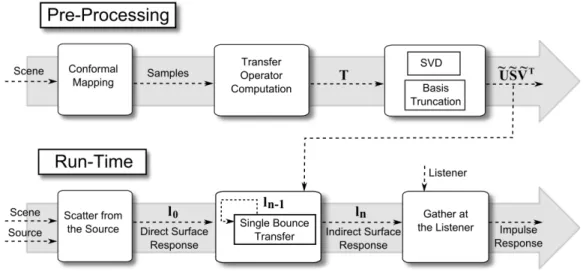
Our algorithm provides two main improvements over the state-of-the-art acoustic radiance transfer algorithms: (a) we decouple the source position from the precom-puted data by computing an acoustic transfer operator; and (b) we use the SVD to compress the transfer operator and quickly compute higher-order reflections. The rest of this chapter details how our algorithm achieves these improvements over the state-of-the-art. Our overall approach is as follows (see Figure 4.1):

• Preprocessing. We sample the surface of the scene and compute a transfer

operator which models one or more orders of diffuse reflections of sound among

1

5286.pdf

Interactive Sound Propagation using

Precomputation and Statistical Approximations

Acknowledgments

Table of Contents

List of Tables

List of Figures

Chapter 1

Introduction

1.1

Applications

1.1.1

Games

1.1.2

Virtual Reality

1.1.3

Architectural Acoustics

1.2

Sound Rendering Pipeline

1.2.1

Sound Synthesis

1.2.2

Sound Propagation

1.2.3

Auralization

1.3

Challenges

1.4

Thesis Statement

1.5

Main Contributions

1.5.1

Direct-to-Indirect Acoustic Radiance Transfer

1.5.2

Compact Acoustic Transfer Operators

1.5.3

Ambient Reverberance and Aural Proxies

1.6

Thesis Outline

Chapter 2

Background

2.1

The Acoustic Wave Equation

2.1.1

Finite Difference Method

2.1.2

Pseudo-Spectral Method

2.1.3

Adaptive Rectangular Decomposition

2.2

The Helmholtz Equation

2.2.1

Finite Element Method

2.2.2

Boundary Element Method

2.2.3

Equivalent Source Method

2.3

Geometric Acoustics

2.3.1

Image Source Method

2.3.2

Stochastic Ray Tracing

2.3.3

Volume Tracing

2.3.4

Diffraction

2.3.5

Acoustic Rendering Equation

2.4

Impulse Responses

2.4.1

Frequency Responses

2.4.2

Echograms

2.5

Auralization

2.5.1

Real-Time Convolution

2.5.2