Yu_unc_0153D_18676.pdf

(1)

STATISTICAL METHODS FOR TOPICS INVOLVING REPEATED MEASURES FOR CATEGORICAL DATA

Jing Yu

A dissertation submitted to the faculty at the University of North Carolina at Chapel Hill in partial fulfillment of the requirements for the degree of Doctor of Public Health in the Department of

Biostatistics in the Gillings School of Global Public Health.

Chapel Hill 2019

(2)

c

2019

Jing Yu

(3)

ABSTRACT

Jing Yu: Statistical Methods For Topics Involving Repeated Measures For Categorical Data

(Under the direction of Gary G. Koch )

Repeated measurement studies involve the collection of inherently multivariate data from the same subject for the same conceptual response variable under two or more experimental and/or observational conditions. The response variables for such studies could be dichotomous,ordered categories, or continuous measurements. Here three topics will be explored: observer variability analysis with standardization for subject variability, conditional log-linear regression for stratified pairs of ordinal responses, and methods for treatment comparisons for subjects with treatments for multiple anatomical regions with ordinal outcomes.

Medical informatics researchers often employ agreement measures to quantify the similarity of ratings by two or more raters in responding to a series of tasks. There is increasing awareness among researchers that the two most appropriate measures of reliability are Kappa and the intraclass correlation coefficient (ICC). When both the row and column marginal distributions are uniform, the interpretation of Kappa is straightforward because the marginals do not influence the level of agreement in any way. El-Khorazaty (El-Khorazaty et al., 2014) described a method of evaluating agreement between two diagnostic contingency tables after adjustment to more clinically relevant marginal distributions using the iterative proportional fitting (IPF) algorithm. We use Weighted Least Squares(WLS) methodology to determine whether the marginal distributions differ between the two treatments. For considering such issues, we not only use the IPF algorithm for adjusting diagnostic contingency tables to uniform marginal totals, as El-Khorazaty et al. did, but also calculate quadratic-weighted adjusted Kappa to compare agreements between the two diagnostic contingency tables. Jackknife confidence intervals (CI) and balanced half-sample variance estimations for average adjusted pairwise Kappas are also addressed for studies with more than two raters.

(4)

of a test treatment to its control. Matching enables elimination of variability in the outcome among the matched sets, thus making it a useful technique when designing a clinical study. A crossover design has another kind of matching. We use the extended Mantel-Haenszel procedure for testing for association, location shift or linear trend progression within the matched pairs. We develop methodology to estimate the treatment effect using the equal adjacent odds ratio model with or without adjustment for covariates. In either type of analysis, log odds ratios and their confidence intervals can be obtained to assess the effects of the treatments. We also can further address extensions of covariance adjustment for ordinal outcomes through using both non-parametric strategies and logistic regression methods. The non-non-parametric methods have essentially no assumptions for a randomized clinical trial, and for a log-linear model can produce results with expected properties.

(5)

ACKNOWLEDGEMENTS

First and foremost, I want to express my deepest gratitude to my advisor, Dr. Gary G. Koch, for his generous support, instructions and deep insights. It has been a great pleasure working with him the past few years. His passion and profession in biostatistics are the leading sources in my growth throughout my dissertation research. I particularly appreciate the generous financial support he provided throughout the years of my graduate study. I really appreciate his kindness and words of encouragement, helping me out during my difficult time. Further, I would like to thank the members of my committee, Drs. Anastasia Ivanova, Lisa M. LaVange, Charles Poole, and John S. Preisser, for their time and their comments which improved the quality of this work.

I would like to sincerely thank Dr. Lisa M. LaVange for the valuable assistance she provided me during my interview process with FDA.

(6)

TABLE OF CONTENTS

LIST OF TABLES . . . . ix

CHAPTER 1: OVERVIEW . . . . 1

1.1 Intraclass Correlation Coefficients (ICC) . . . 2

1.1.1 Reliability Theory . . . 2

1.1.2 Marginal Dependency Of ICC . . . 3

1.2 Kappa Statistics . . . 3

1.2.1 Cohen’s Kappa Coefficient . . . 3

1.2.2 Weighted Kappa Coefficient . . . 6

1.2.3 95% Confidence Interval For Kappa . . . 8

1.2.4 Marginal Dependency Of Kappa . . . 10

CHAPTER 2: OBSERVER VARIABILITY ANALYSIS WITH STANDARDIZATION FOR SUBJECT VARIABILITY . . . . 27

2.1 Overview . . . 27

2.2 Methods . . . 27

2.2.1 Iterative Proportional Fitting (IPF) Algorithm . . . 27

2.2.2 Intraclass Correlation Coefficients (ICC) . . . 28

2.2.3 Quadratic Weighted Kappa . . . 28

2.3 Examples . . . 28

2.4 Discussions . . . 38

CHAPTER 3: CONDITIONAL LOG-LINEAR REGRESSION FOR STRATIFIED PAIRS OF ORDINAL RESPONSES . . . . 39

3.1 Overview . . . 39

3.2 Methods . . . 40

(7)

3.2.2 Randomization-Based Analysis Of Covariance (RANCOVA) . . . 41

3.3 Examples . . . 42

3.3.1 Clinical Trial Example For Improvement Of A Skin Condition . . . 42

3.3.2 Clinical Trials Example From El-Khorazaty Paper . . . 46

3.3.3 Two Period Crossover Study For Patients With Recurrent Pain . . . 49

3.3.4 Crossover Clinical Trial Example For Patients With Os-teoarthritis . . . 51

CHAPTER 4: METHODS FOR TREATMENT COMPARISONS FOR ORDINAL OUTCOMES FOR MULTIPLE ANATOMICAL REGIONS . . . . 60

4.1 Overview . . . 60

4.2 Methods . . . 61

4.2.1 Extended Cochran-Mantel-Haenszel (CMH) Method . . . 61

4.2.2 Randomization-Based Analysis Of Covariance (RANCOVA) . . . 63

4.3 Examples . . . 64

4.3.1 Clinical Trial Example in Ophthalmology . . . 64

4.3.2 Clinical Trial Example for Seborrheic Dermatitis . . . 70

CHAPTER 5: CONCLUSIONS AND FUTURE DIRECTIONS . . . . 77

5.1 Agreement Measure . . . 77

5.2 Matched Pairs Study . . . 79

5.3 Multiple Anatomical Regions Affected Study . . . 80

APPENDIX 2: APPENDIX FOR CHAPTER 2 . . . . 82

(8)

LIST OF TABLES

1.1 Generic 2×2 table format for assessing agreement between two

raters classifying N units into same 2 categories . . . 5

1.2 Frequency distributions of primary efficacy results . . . 12

1.3 Observed and adjusted estimates of agreement, corresponding stan-dard errors and 0.95 confidence intervals for Study 5131. . . 14

1.4 Observed and adjusted estimates of agreement, corresponding stan-dard errors and 0.95 confidence intervals for Study 5132. . . 15

1.5 Test of marginal homogeneity in two treatment groups for both studies, using weighted least squares methodology. . . 16

1.6 Frequency distributions of MS diagnosis by two neurologists: Win-nipeg and New Orleans patients. . . 17

1.7 Test of marginal homogeneity in two neurologists for both Winnipeg and New Orleans patients, using weighted least squares methodology. . . 18

1.8 Observed and adjusted estimates of agreement, corresponding stan-dard errors and 0.95 confidence intervals. . . 19

1.9 Frequency distributions of diagnostic categories of the slides from uterine cervix by seven pathologists using Five-Point or Two-Point ordinal scale. . . 20

1.10 Statistical tests of marginal homogeneity using Dichotomous scale(with D.F.=1) and Four-Point scale(with D.F.=3) between pairwise pathol-ogists. . . 22

1.11 Ordinary and adjusted Kappa (Standard Error) for pairs of pathol-ogists using Dichotomous scale via El-Khorazaty formula. . . 24

1.12 Uniformly distributed proportions in agreement for binary classifications. . . 25

1.13 Jackknife confidence interval (CI) for average adjusted pairwise Kappas. . . 26

2.1 Distribution of master grades with N=300 . . . 30

2.2 Cases pertaining to different levels of disagreement . . . 31

2.3 Mean ICC (and interdecile range) across 10000 simulations of uni-form, convex and concave distributions with N=300 and samples of at least size n=80 form extreme and mild concave and convex distributions . . . 32

2.4 Intraclass Correlation (ICC) of ratings on the same subject (Sub-jects=300, Raters=8) . . . 33

2.5 Average pairwise quadratic weighted Kappa (Subjects=300, Raters=8) . . . 33

(9)

2.7 Distribution of raters’ grades for clinical data (N=400) of the 5

photonumeric scales. . . 34

2.8 Estimates for average ordinary pairwise Kappas and average qua-dratic weighted pairwise Kappas (for clinical data). . . 36

2.9 Estimates for average adjusted pairwise Kappas with corresponding standard error (SE) from Balanced Repeated Replication (BRR) and Jackknife confidence interval (CI) (for clinical data). . . 36

2.10 Estimates for average adjusted quadratic weighted pairwise Kappas with corresponding standard error (SE) from Balanced Repeated Replication (BRR) and Jackknife confidence interval (CI) (for clini-cal data). . . 37

2.11 ICC of paired ratings on the same subject, subject variance ˆσ2 s, rater variance ˆσ_r2, and mean square errors ˆσ2_e estimates for 5 scales from two-way Analysis of Variance (ANOVA) (for clinical data). . . 37

3.1 Clinic Pairs Breakdown . . . 43

3.2 (0,1) Configuration Table (15) . . . 43

3.8 P values, odds ratio and corresponding 95% confidence interval for each variable, interaction terms and Goodness-of-Fit (Deviance) in different models for all patients. . . 46

3.9 Frequency distributions of primary efficacy results . . . 47

3.10 Equal adjacent odds ratio and corresponding 95% confidence interval from Logistic Regression forStudy∗Groupfor each treatment group of Study 5131 and Study 5132. . . 47

3.11 P values, odds ratio and corresponding 95% confidence interval for each variable, interaction terms and Goodness-of-Fit (Deviance) in different models for all patients in both treatment groups of Study 5131 and Study 5132. . . 48

3.12 Data from a crossover clinical trial for the comparison of treatments for relief of a recurrent pain condition. . . 49

(10)

3.14 Goodness-of-Fit (Deviance) for models for both sequences and p-values, estimates and corresponding standard errors (SE) for

treat-ments ( T vs. P ) and periods ( 1 vs. 2 ) effects. . . 50 3.15 Data from a crossover clinical trial for patients with osteoarthritis

with single imputation for missing data. . . 52 3.16 Means, standard errors, and p-values for (visit 2 - visit 4) differences

of continuous baseline measurements with (visit 3 - visit 5)6= 0 for

trichotomous response, with single imputation for missing data. . . 52 3.17 Goodness-of-Fit statistics (Deviance and corresponding p value) from

Logistic Regression for equal adjacent odds models for comparing treatment periods in sequences, estimates and standard errors (SE),

with single imputation for missing data. . . 52 3.18 Goodness-of-Fit (Deviance) for models for both sequences and

p-values, estimates and corresponding standard errors (SE) for treat-ments ( Arthrotec vs. Acetaminophen ) and periods ( 1 vs. 2 ) effects, with/without adjusting for the differences between baseline

measurements, with single imputation for missing data. . . 53 3.19 Estimates and standard errors (SE) from Logistic Regression for

equal adjacent odds models for comparing treatment periods in sequences, with/without adjusting for the baseline measurements,

with multiple imputation for missing data. . . 54 3.20 Estimates, corresponding standard errors (SE) and p-values for

treatments ( Arthrotec vs. Acetaminophen ) and periods ( 1 vs. 2 ) effects, for models, with/without adjusting for the baseline

measurements, and with multiple imputation for missing data. . . 54 3.21 Estimates, corresponding standard errors (SE) and p-values for

treatments ( Arthrotec vs. Acetaminophen ) and periods ( 1 vs. 2 ) effects, using RANCOVA method based on Appendix 3.5.2, adjusting for the baseline measurements, and with single imputation

for missing data. . . 55 3.22 Estimates, corresponding standard errors (SE) and p-values for

treatments ( Arthrotec vs. Acetaminophen ) and periods ( 1 vs. 2 ) effects, using RANCOVA method based on Appendix 3.5.2, adjusting for the baseline measurements, and with multiple imputation for

missing data. . . 56 3.23 Estimates, corresponding standard errors (SE) and p-values for

treatments ( Arthrotec vs. Acetaminophen ) and periods ( 1 vs. 2 ) effects, using RANCOVA method based on Appendix 3.5.3, adjusting for the baseline measurements, and with single imputation

for missing data. . . 57 3.24 Estimates, corresponding standard errors (SE) and p-values for

treatments ( Arthrotec vs. Acetaminophen ) and periods ( 1 vs. 2 ) effects, using RANCOVA method based on Appendix 3.5.3, adjusting for the baseline measurements, and with multiple imputation for

(11)

3.25 Estimates, corresponding standard errors (SE) and p-values for treatments ( Arthrotec vs. Acetaminophen ) and periods ( 1 vs. 2 ) effects, using RANCOVA method based on Appendix 3.5.4, adjusting for the baseline measurements, and with single/multiple

imputation for missing data. . . 58

4.1 Number of eyes with not favorable or favorable outcome for (>1 vs. ₆1) dichotomy in randomized clinical trial in ophthalmology,

cross-classified by treatments and number of enrolled eyes. . . 65 4.2 Sum of eyes for sum of dichotomous specifications for not favorable

or favorable outcome as (>1 vs. ₆ 1) and (>2 vs. ₆2),

cross-classified by treatments and number of enrolled eyes. . . 66 4.3 Stratified estimators for extent of good outcome, standard error

(SE) and 0.95 confidence interval (CI), regardless of whether the null hypothesis applies (re proportions with good outcome as p∗ij

and ¯y∗∗i=P2j=1p∗ij in Appendix 4.5.4). . . 67

4.4 Stratified estimators for extent of good outcome, standard error (SE) and 0.95 confidence interval (CI), regardless of whether the null hypothesis applies (re CMH weighted averages ˜p∗ij and ˜y∗∗i = P2

j=1p∗˜ij in Appendix 4.5.4). . . 68

4.5 Estimated treatment effects and 0.95 confidence interval (CI) by

%NParCov4 method. . . 69 4.6 Number of anatomical regions with not favorable or favorable

out-come (for _> 2 vs. ₆ 1) dichotomy by treatment and number of

anatomical regions for patients with seborrheic dermatitis. . . 71 4.7 Sum of anatomical regions for sum of dichotomous specifications for

not favorable or favorable outcome as (>2 vs. 61) and (>3 vs.

62) by treatment and number of anatomical regions for patients

with seborrheic dermatitis. . . 72 4.8 Stratified estimators for extent of good outcome, standard error

(SE) and 0.95 confidence interval (CI), regardless of whether the null hypothesis applies (re proportions with good outcome as p∗ij

and ¯y∗∗i=P2j=1p∗ij in Appendix 4.5.4). . . 73

4.9 Stratified estimators for extent of good outcome, standard error (SE) and 0.95 confidence interval (CI), regardless of whether the null hypothesis applies (re CMH weighted averages as ˜p∗ij and

˜

y∗∗i =P2j=1p∗˜ ij in Appendix 4.5.4). . . 74

4.10 Estimated treatment effects and 0.95 confidence interval (CI) by

(12)

CHAPTER 1: OVERVIEW

Medical informatics researchers often employ agreement measures to quantify the similarity of ratings by two or more raters in responding to a series of tasks. Human judgment is at once a significant strength as well as a weakness in this research. Consider studies for behavior observation and clinical diagnosis, for example. People are capable of integrating a complex set of cues to arrive at psychologically informed judgments. At the same time, these judgments are imperfect; they are influenced by the characteristics of the raters themselves (e.g., experiences, conscientiousness) as well as random error. Even when raters use the same set of rules, they often produce different assessments. Careful training can reduce but not eliminate differences among raters. Accordingly, establishing and reporting sufficient interrater agreement is essential in rating studies. Researchers must be able to show that the judgments of behavior and diagnoses are sufficiently reproducible among different raters to be taken as scientifically objective observations. Furthermore, obtaining substantial interrater agreement is a critical step in establishing the reliability and validity of rating data.

(13)

1.1 Intraclass Correlation Coefficients (ICC)

1.1.1 Reliability Theory

For a group of measurements, the total variance (σ2

T) in the data can be viewed as being due

to true score variance (σ2

t) and error variance (σe2). Similarly, each observed score is composed of

the true score and error. The theoretical true score of an individual reflects the mean of an infinite number of scores from a subject, whereas error equals the difference between the true score and the observed score. If we make a ratio of the σ2_t to theσ2_T of the observed scores, whereσ2_T equalsσ_t2 plusσ2_e, we have the following reliability coefficient: R= σ2t

σ2

t+σ2e

. The closer this ratio is to 1.0, the higher the reliability and the lower theσ_e2. Since we do not know the true score for each subject, the counterpart ofσ_t2 is based on between subjects variability. In this context, reliability is formally defined as follows: Reliability = _{BetweenSubjectsV ariability}BetweenSubjectsV ariability₊_error, and it is an intraclass correlation coefficient (ICC).

The ICC is a relative measure of reliability in that it is a ratio of variance derived from Analysis of Variance (ANOVA), is unitless, and is more conceptually akin to R2 from regression than to the Pearson correlation r. The ICC can theoretically vary between 0 and 1.0, where an ICC of 0 indicates no reliability, and an ICC of 1.0 indicates perfect reliability. The relative nature of the ICC is reflected in the fact that the magnitude of ICC depends on the between subjects variability. That is, if subjects differ little from each other, ICC values are small even if trial-to-trial variability is small. If subjects differ from each other a lot, ICC can be large even if trial-to-trial variability is large. Thus, the ICC for a measurement is context specific.

Error is typically considered as being of 2 types: systematic error (e.g., bias) and random error. Total error reflects both systematic error and random error. Systematic error includes both constant error and bias. Constant error affects all scores equally, whereas bias is systematic error that affects certain scores differently than others. In contrast, random error refers to sources of error that are due to chance factors. Thus, we can have R = σt2

σ2

t+σ2se+σ2re

(14)

1.1.2 Marginal Dependency Of ICC

An issue of concern for interpreting the ICC is that it is dependent of σ2_t for subject variability, since it can understate reliability when σ_t2 is relatively small regardless of how small σ_e2 is. This issue is addressed in Mehta et al., 2018 through a sampling method that produces a larger value of σ_t2 for an internal population with larger sampling variability making for an alternative population with larger sampling variability. Additional discussion of considerations addressed by Mehta et al. will be provided in Chapter 2.

1.2 Kappa Statistics

1.2.1 Cohen’s Kappa Coefficient

A chance-corrected measure introduced by Scott (Scott, 1955), was extended by Cohen (Cohen, 1960) and has come to be known as Cohen’s Kappa. It springs from the notion that the observed cases of agreement include some cases for which the agreement was by chance alone. Cohen assumed that there were two raters, who ratensubjects into one of m mutually exclusive and exhaustive nominal categories. The raters operate independently; however, there is no restriction on the marginal distribution of the ratings for either rater. Letpij be the proportion of subjects that were

placed in thei, jth cell, i.e., assigned to the ith category by the first rater and to the jth category by the second rater (i, j = 1, ..., m). Also, let pi.=Pmj=1pij denote the proportion of subjects placed

in the ith row (i.e., the ith category by the first rater), and letp.j =Pmi=1pij denote the proportion

of subjects placed in thejth column (i.e., thejth category by the second rater). Then, the Kappa coefficient proposed by Cohen is ˆκ = po−pc

1−pc , where po =

Pm

i=1pii is the observed proportion of

agreement, which is the probability that two raters both endorsed the presence or absence of a behavior or diagnosis; and pc=Pmi=1pi.p.i is the proportion of agreement expected by chance. The

Kappa statistic thus ranges between −pc

(15)

that the distribution of proportions over the m categories for the population is known, and is equal for the two raters. Therefore, if the two raters are interchangeable, in the sense that the marginal distributions are identical, then Cohen’s and Scott’s measures are equivalent. To determine whether ˆ

κ differs significantly from zero, one could use the asymptotic variance formula given by Fleiss et al. (Fleiss et al., 1969) for the general m×m table. Under the hypothesis ofκ= 0, the estimated large-sample variance of ˆκ is given byV ar[κˆ =

Pm

i=1pii[1−(pi.+p.i)]

2₊P

i6=jpij×(p.i+pj.)

2₋_p2

c

N(1−pc)2 for sample sizeN (Fleiss et al., 2013). Assuming that √κˆ

\ V arˆκ

follows a normal distribution, one can test the hypothesis of chance agreement by reference to the standard normal distribution.

Landis and Koch (Landis and Koch, 1977b) have characterized different ranges of values for Kappa with respect to the degree of agreement they suggest. Although these original suggestions were admitted to be "clearly arbitrary", they have become incorporated into the literature as standards for the interpretation of Kappa values, and El-Khorazaty et al. (El-Khorazaty et al., 2014) have provided additional clarification for their rationale. For most purposes, values greater than 0.75 or so may be taken to represent excellent agreement beyond chance, values below 0.40 or so may be taken to represent poor agreement beyond chance, and values between 0.40 and 0.75 may be taken to represent fair to good agreement beyond chance.

(16)

Table 1.1: Generic 2×2 table format for assessing agreement between two raters classifyingN units into same 2 categories

Rater B

Yes No Total

Rater A Yes x11 x12 g1

No x21 x22 g2

Total f1 f2 N

Cohen introduced Kappa as an alternative to such categorical association statistics as the χ2 , noting that association statistics are increased by greater than chance disagreements as much as agreements. Thus, Kappa was formulated to exclusively reflect chance corrected agreement rather than degree of association. Cohen’s Kappa provides a correction for agreement by chance based on the obtained distributions of two raters rather than the hypothetical random behavior of raters under a predetermined set of conditions. The calculation of chance agreement for Kappa depends on the obtained marginal frequencies (i.e., the row and column totals in Table 1.1). Symmetrically imbalance between the two row marginals and between the two column marginals increase the estimate of chance agreement. This feature explains Kappa’s base rate sensitivity, as low base rates produce symmetrically unbalanced marginals; more of the ratings fall into the behavior or diagnosis "No" than "Yes" category.

(17)

for other populations.

1.2.2 Weighted Kappa Coefficient

Often situations arise when certain disagreements between two raters are more serious than others. Cohen (Cohen, 1968) introduced an extension of Kappa called the weighted Kappa statistic ( ˆκw), to measure the proportion of weighted agreement corrected for chance. Either degree of

disagreement or degree of agreement is weighted, depending on what seems natural in a given context. Cohen (1968) introduced weights in the formulation of the agreement coefficient leading to the weighted Kappa coefficient. Although the weights can be arbitrarily chosen, those introduced by Cicchetti and Allison (Cicchetti and Allison, 1971) and by Fleiss and Cohen (Fleiss and Cohen, 1973) are the most commonly used. The former depend linearly on the distance between the classification made by the two raters, while the latter depend quadratically on that distance. Quadratic weights are the most popular because of their practical interpretation. Cohen (1968) and Schuster (Schuster, 2004) showed that the quadratic-weighted Kappa coefficient is asymptotically equivalent to the intraclass correlation coefficient under a two-way ANOVA model. In other words, the quadratic-weighted Kappa coefficient compares the variability between the pairs of ratings for subjects to the total variability. Similarly to Cohen’s Kappa coefficient, the linear-weighted Kappa coefficient is a weighted average of individual Kappa coefficients obtained on 2×2 tables constructed by collapsing the first M categories and last m−M categories ( M = 1, ..., m−1) of the original m×m classification table.

The statistic ˆκw, provides for the incorporation of ratio-scaled degrees of disagreement (or

agreement) to each of the cells of them×m table of joint assignments such that disagreements of varying gravity (or agreements of varying degree) are weighted accordingly. The nonnegative weights are set prior to the collection of the data. Since the cells are scaled for degrees of disagreement (or agreement), some of them are not given full disagreement credit. However, ˆκw, like the unweighted

ˆ

κ, is fully chance-corrected.

Assuming thatwij represents the weight for agreement assigned to thei, jth cell (i, j= 1, ..., m),

the weighted Kappa statistic is given by ˆκw = Pm

i=1 Pm

j=1wijpij− Pm

i=1 Pm

j=1wijpi.p.j

1−Pm i=1

Pm

j=1wijpi.p.j

, where 0≤wij ≤1

with wii= 1. Note that the unweighted Kappa is a special case of ˆκw with wij = 1 for i=j and

(18)

assigned the numerical values 1,2, ..., m, and if wQ,ij= 1− (i−j) 2

(m−1)2 for quadratic weights, then ˆκw

can be interpreted as an intraclass correlation coefficient for a two-way ANOVA computed under the assumption that the n subjects and the two raters are random samples from populations of subjects and raters, respectively (Fleiss and Cohen, 1973).

Linear-Weighted Kappa CoefficientCicchetti and Allison (1971) proposed linear weights of the formwL,ij = 1−

|i−j|

(m−1), with the observed linear-weighted disagreement being the mean distance (number of categories) between the classifications made by the two raters. In the same way, the expected linear-weighted disagreement is the mean distance expected by chance. The linear-weighted Kappa therefore compares the mean distance between the classifications made by the two raters to the mean distance expected by chance and can thus be interpreted as the chance-corrected mean distance between the two classifications: κL = 1− _{M eanDistanceBetweenT heT woClassif icationsExpectedByChance}M eanDistanceBetweenT heT woClassif ications .

IfκL=x , the observed mean distance between the two raters’ classifications is (1−x) times the

mean distance expected by chance. Perfect agreement (κL = 1) is obtained when the observed

mean distance between the two classifications is null, i.e., there is no disagreement. A value of zero indicates that the observed mean distance is only to be expected by chance, while negative values express that the observed mean distance is larger than the mean distance expected by chance.

Quadratic-Weighted Kappa Coefficient Fleiss and Cohen (1973) used quadratic weights wQ,ij = 1 − (i−j)

2

(m−1)2, and so the observed quadratic-weighted disagreement is the moment of

inertia of the distance distribution between the two raters’ classifications about the axis formed by the agreement cells. It, therefore, gives a measure of concentration (or variability) of the distance distribution around 0. In the same way, the expected quadratic-weighted disagreement corresponds to the concentration expected by chance. The quadratic-weighted Kappa therefore compares the observed concentration of the distance distribution between two raters’ classifications about 0 to the concentration expected by chance. It can be interpreted as the chance-corrected measure of concentration about 0 of the distance distribution between the two raters’ classifications: κQ = 1− ConcentrationAboutZeroOf T heDistanceBetweenT heT woClassif ications_{ConcentrationAboutZeroExpectedByChance} . If κQ = x, the observed

concentration of the distance distribution between the two raters’ classifications about 0 is (1−x) times that expected by chance. Perfect agreement (κQ = 1) means that the moment of inertia is 0,

(19)

values correspond to a distribution of the distance between the two raters’ classifications being more dispersed than what is expected by chance.

Classically, Cohen’s Kappa coefficient is used on nominal scales and weighted agreement coeffi-cients on ordinal scales. Cohen’s Kappa coefficient can, however, be used for ordinal scales when all disagreements are assumed to be equally important. For example, in diagnostic decision making, this could be in terms of consequences for the patient. When disagreements cannot be considered as having the same importance, reporting both linear- and quadratic-weighted Kappa coefficients will provide more information on the distribution of disagreement than reporting one coefficient alone. Indeed, as a general statistical principle, the use of a position and a variability parameter better describe a distribution than the use of one parameter alone. If only one coefficient has to be chosen, the linear-weighted Kappa coefficient is sometimes advised because (1) a position parameter is first used to summarize a statistical distribution, (2) the interpretation of the linear-weighted Kappa in terms of mean distance between the two raters’ classifications is very simple, (3) the linear-weighted Kappa coefficient (a position parameter) is less influenced by the choice of the number of categories of the scale than the quadratic-weighted Kappa coefficient (a variability parameter) (Brenner and Kliebsch, 1996), and (4) the quadratic-weighted Kappa coefficient can possess possibly unappealing mathematical properties (Warrens, 2012), through the value of quadratically weighted Kappa not depending on the value of the center cell of the agreement table. Thus, for the table with skewed marginal totals, quadratically weighted Kappa cannot discriminate between agreements. Nevertheless, quadratic-weighted Kappa is ICC’s counterpart.

1.2.3 95% Confidence Interval For Kappa

(20)

crude approximation only to the variance of Kappa (Altman, 1990), V ar(κ) = po×(1−po)

N×(1−pc) . Thus, the standard error of Kappa is defined as the square root of its variance. Since Kappa follows an approximate normal distribution, a 95% confidence interval for Kappa can be estimated as κ±1.96×SE(κ). For testing the hypothesis that the underlying value of Kappa (either overall or for a single category) is equal to a prespecified value Kappa other than zero, Fleiss (Fleiss et al., 2013) showed that the appropriate standard error of ˆκ is estimated by ˆse(ˆκ) = ₍₁A₋+_pB−C

e) √

n, where the

overall proportion of chance-expected agreementpe =Pki=1pi.p.i,A=Pki=1pii[1−(pi.+p.i)(1−ˆκ)]2,

B = (1−ˆκ)2P P

i6=jpij(p.i+pj.)2, and C = [ˆκ−pe(1−ˆκ)]2. The hypothesis that Kappa is the

underlying value would be rejected if the critical ratio z= |_seˆκ_ˆ−_(ˆ_κκ₎| were found to be significantly large from tables of the normal distribution. For positive values of Kappa, if the lower boundary crosses zero, then agreement is not significantly different from chance (at an arbitrary 5% level). If the lower boundary is above zero then agreement is significantly above chance.

Virtually all related textbooks which include Kappa discuss the statistical test of the null hypothesis for Kappa and the estimation of the confidence interval (CI) based on the normal distribution. Although the normal theory procedure is reliable for testing of null hypotheses, the procedure is often not reliable for constructing a confidence interval, particularly when Kappa exceeds 0.50. As the Kappa coefficient is bounded by 1 (perfect agreement), its sampling distribution can be highly skewed when strong agreement or reproducibility exists. A better alternative to determine the confidence interval of Kappa is therefore based on the empirical sampling distribution generated by the computer intensive bootstrap resampling method or by the jackknife method (Efron and Tibshirani, 1986) (Hellmann and Fowler, 1999).

Bootstrap Confidence IntervalsFor the Contingency table (CT), generated by a sample from the population, 1000 independent bootstrap re-samplesX₁∗, X₂∗, ..., X₁₀₀₀∗ of sizeN are generated. Each bootstrap re-sample X∗ = (x∗₁, x∗₂, x∗₃, ..., x∗_N) is obtained by randomly sampling 1000 times, with replacement, from the original data set X = (x1, x2, x3, ..., xN). To obtain the bootstrap

(21)

in the ordered bootstrap pairwise agreement measures are chosen.

Jackknife Confidence Intervals The delete-one jackknife relies on resamples that omit one entity of the sample at a time, where entities are those individuals that are randomly sampled from the population. A pseudo-values approach is used to calculate the jackknife CIs. For an estimator S, thekth pseudo-value of S is calculated asP Sk =N S−(N −1)Sk, where Sk is the estimated

value for the sample with the kth data point deleted. The jackknife CI was then calculated as CIJ(95%) =P S±2

q_var

N , where var=

1

N−1

PN

k=1(P Sk−P S)2 , andP S = _N1 PNk=1P Sk.

1.2.4 Marginal Dependency Of Kappa

It is often of interest to measure the agreement between raters when an outcome is nominal or ordinal. In such scale reliability studies, although there is no guidance regarding the number of subjects in each grade of the scale, the Kappa statistic is highly sensitive to the distribution of the marginal totals and can produce results that are puzzling (Kim et al., 2004) (Cohen, 1960) (Vach, 2005) (Byrt et al., 1993). The interpretation of Kappa should be contingent on the raters’ marginal distributions, and ignoring this information may induce inaccurate and potentially misleading conclusions. The main point is that the level of agreement between two classifications is systematically restricted, bounded from below and above, by the level of agreement between the two raters’ marginal distributions: The more similar the two distributions are, the more likely it is that Kappa will have 1.0 as its upper bound. Conversely, the more different they are, the more likely it is that Kappa will have an upper bound that is lower than 1. Consequently, comparing agreement measures across different tables can be problematic. Also, evaluations of scales using subjects that are homogeneous tend to have poorer κ, weightedκ and ICC values than those that utilize more heterogeneous distributions of subjects. Thus, it may be critical to assess reliability of a scale with an equally likely (uniform) distribution of subjects, since it has a more standardized setting.

(22)

(23)

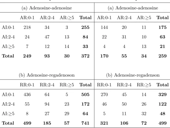
Table 1.2: Frequency distributions of primary efficacy results

For Study 5131 For Study 5132

(a) Adenosine-adenosine (a) Adenosine-adenosine

AR:0-1 AR:2-4 AR:≥5 Total AR:0-1 AR:2-4 AR:≥5 Total

AI:0-1 218 34 3 255 144 20 11 175

AI:2-4 24 47 13 84 22 31 10 63

AI:≥5 7 12 14 33 4 4 13 21

Total 249 93 30 372 170 55 34 259

(b) Adenosine-regadenoson (b) Adenosine-regadenson

RR:0-1 RR:2-4 RR:≥5 Total RR:0-1 RR:2-4 RR:≥5 Total

AI:0-1 436 64 5 505 270 45 14 329

AI:2-4 55 94 23 172 46 50 26 122

AI:≥5 8 27 29 64 5 11 32 48

Total 499 185 57 741 321 106 72 499

From Table 1.2, the number of patients with the least severe condition (i.e.,0-1) is substantially greater than those with more severe status, with that making agreement under a more equal distribution for the categories of more interest than the usual methodology for agreement allowed. El-Khorazaty (El-Khorazaty et al., 2014) standardized the population distribution of subjects using the iterative proportional fitting algorithm. They estimated the cell counts in the cells of a contingency table while maintaining fixed marginal totals. Each row of the original distribution of cell counts in a two-way contingency table is proportionally adjusted to have its total equal the specified marginal row total distribution, and each column is proportionally adjusted to have its total equal the specified marginal column total distribution. This process is repeated iteratively until a specified level of convergence is reached. For a 3×3 contingency table for evaluating the agreement between two diagnostic tests, the sample proportions arepij =nij/N , where nij is the

(24)

distributions to uniform distributions makes ˜A= (˜n11+˜n22_N+˜n33) = (˜p11+ ˜p22+ ˜p33), the agreement without chance correction, where the ˜nii are the modified frequencies from adjustment to uniform

marginal distributions by IPF, and the ˜pii= (˜nii/N). Then the adjusted Kappa ˜κ is calculated as:

˜ κ=

˜

n_11+˜n_22+˜n₃₃ N −1/3

1−1/3 =

3( ˜p11+ ˜p22+ ˜p33)−1

2 = (3 ˜A−1)/2. In this case, there are uniform distributions for the row and column totals. For the purposes of IPF and the asymptotic covariance matrix of the estimators, there is transformation of the countsnij of each cell and proportionspij = (nij/N).

In order to preserve the observed association structure, as measured by odds ratios formed by pairs of rows and pairs of columns, the algorithm is started by using the observed cell proportions as the initial values, ˜p(0)_ij so that ˜p(0)_ij = pij. The IPF algorithm proceeds as: ˜p(ijt) = ˜p

(t−1)

ij (

1/3 ˜

p(_it₊−1))

, ˜p(_ijt+1) = ˜p(_ijt)(1/3 ˜

p(₊t_j)) for t= 1,3,5, ... At the end of each odd numbered step, all row totals equal

1/3. At the end of each even-numbered step, all column totals equal 1/3. When all nij > 0,

the algorithm converges after several iterations with all row and column totals equaling 1/3 (El-Khorazaty et al., 2014). A consistent estimator for the asymptotic covariance matrix of the estimators, ˜

p= (˜p11,p˜12,p˜13, ....,p˜33)0 is given by V(˜p) as: V(˜p) =K0[KD−p˜1K0]−1KD−p1K0[KD

−1 ˜

p K0]−1K/N ,

where the matrix

K4×9 =

         

1 −1 0 −1 1 0 0 0 0 1 −1 0 0 0 0 −1 1 0 1 0 −1 −1 0 1 0 0 0 1 0 −1 0 0 0 −1 0 1

         

For the calculations,p= (p11, p12, p13, ..., p33)0 is the

vector of original table cell proportions, ˜p is the vector of fitted cell proportions, Dp is the diagonal

matrix withpas diagonal elements, andDp˜is the diagonal matrix with ˜pas diagonal elements. From V(˜p) , a consistent estimator for the variance of ˜AisV( ˜A) as: V( ˜A) =

1 0 0 0 1 0 0 0 1

V(˜p)

1 0 0 0 1 0 0 0 1

0 _{, It follows that ( ˜}_A_±_1.96q_V_{( ˜}_{A)) provides a 95% CI for the}

(25)

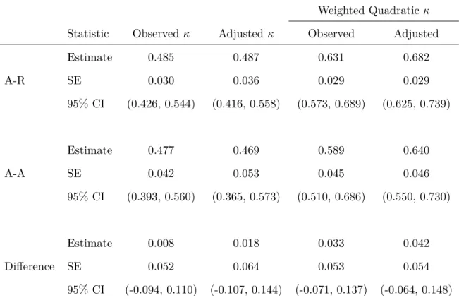
Table 1.3: Observed and adjusted estimates of agreement, corresponding standard errors and 0.95 confidence intervals for Study 5131.

Weighted Quadraticκ Statistic Observed κ Adjustedκ Observed Adjusted

Estimate 0.485 0.487 0.631 0.682

A-R SE 0.030 0.036 0.029 0.029

95% CI (0.426, 0.544) (0.416, 0.558) (0.573, 0.689) (0.625, 0.739)

Estimate 0.477 0.469 0.589 0.640

A-A SE 0.042 0.053 0.045 0.046

95% CI (0.393, 0.560) (0.365, 0.573) (0.510, 0.686) (0.550, 0.730)

Estimate 0.008 0.018 0.033 0.042

Difference SE 0.052 0.064 0.053 0.054

(26)

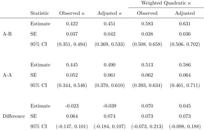
Table 1.4: Observed and adjusted estimates of agreement, corresponding standard errors and 0.95 confidence intervals for Study 5132.

Estimate 0.422 0.451 0.583 0.631

A-R SE 0.037 0.042 0.038 0.036

95% CI (0.351, 0.494) (0.369, 0.533) (0.508, 0.658) (0.506, 0.702)

Estimate 0.445 0.490 0.513 0.586

A-A SE 0.052 0.061 0.062 0.064

95% CI (0.344, 0.546) (0.370, 0.610) (0.393, 0.634) (0.461, 0.711)

Estimate -0.023 -0.039 0.070 0.045

Difference SE 0.064 0.074 0.073 0.073

95% CI (-0.147, 0.101) (-0.184, 0.107) (-0.073, 0.213) (-0.098, 0.188) * A-R is Adenosine-regadenoson treatment group; A-A is Adenosine-adenosine treatment group.

(27)

the two treatments. From Table 1.5, marginal distributions are reasonably similar for the two treatments in both studies, although less so for Study 5132. El-Khorazaty didn’t address that issue in their paper. But there is not really much difference between the marginal distributions for either study.

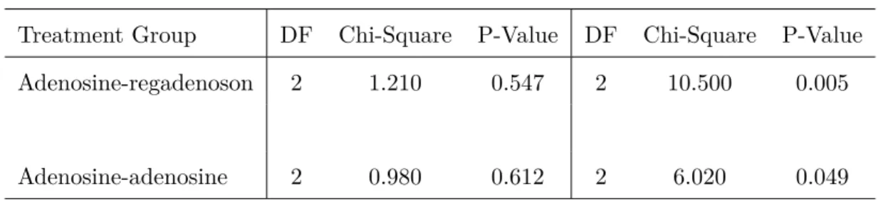
Table 1.5: Test of marginal homogeneity in two treatment groups for both studies, using weighted least squares methodology.

For Study 5131 For Study 5132

Treatment Group DF Chi-Square P-Value DF Chi-Square P-Value

Adenosine-regadenoson 2 1.210 0.547 2 10.500 0.005

Adenosine-adenosine 2 0.980 0.612 2 6.020 0.049

From Table 1.5, we noted that the marginal distributions in the two treatment groups are essentially the same for Study 5131, but somewhat different for Study 5132. In the Study 5132, the number of patients with the most severe condition (≥5) is substantially greater by the second diagnostic scan for both treatment groups. For considering such issues, we calculate quadratic-weighted adjusted Kappa to compare agreements between the two diagnostic contingency tables. We use the IPF algorithm for adjusting diagnostic contingency tables to uniform marginal totals, as El-Khorazaty did. The quadratic-weighted adjusted Kappa ˜κQ is obtained using the relationship ˜AQ =

1 3₄ 0 3₄ 1 3₄ 0 3₄ 1

(˜p11,p˜12,p˜13, ....,p˜33), ˜κQ = ( ˜AQ

−2/3)

(1/3) and its estimated variance is V(˜κQ) = 9V( ˜AQ). We obtain higher agreement levels in both treatment groups for the two studies

by weighted adjusted Kappas with smaller (or similar) standard errors, and results are shown in Table 1.3 and Table 1.4.

(28)

four-point ordinal scale for Multiple Sclerosis (MS) diagnostic classes: (1) certain MS; (2) probable MS; (3) possible MS; (4) doubtful, unlikely or definitely not MS. In order to evaluate agreement between the diagnosticians, the Winnipeg neurologist then reviewed and classified each of the New Orleans patient records, and vice versa. The data resulting from these diagnoses and their review are presented in Table 1.6.

Table 1.6: Frequency distributions of MS diagnosis by two neurologists: Winnipeg and New Orleans patients.

Subgroup 1 Subgroup 2

Winnipeg patients(n=149) New Orleans patients(n=69)

New Orleans neurologists (1)

Winnipeg neurologists (2)

Total

Winnipeg neurologists (2)

Total

1 2 3 4 1 2 3 4

1 38 5 0 1 44 5 3 0 0 8

2 33 11 3 0 47 3 11 4 0 18

3 10 14 5 6 35 2 13 3 4 22

4 3 7 3 10 23 1 2 4 14 21

Total 84 37 11 17 149 11 29 11 18 69

* Diagnostic categories: (1) certain MS; (2) probable MS; (3) possible MS; (4) doubtful, unlikely or definitely

not MS.

(29)

(χ2= 10.54). These results suggested that significant inter-observer bias existed between the two neurologists in their overall usage of the diagnostic classification scale.

Table 1.7: Test of marginal homogeneity in two neurologists for both Winnipeg and New Orleans patients, using weighted least squares methodology.

Neurologists DF Chi-Square P-Value (1)Winnipeg patients 3 58.470 <0.001

(2)New Orleans patients 3 10.540 0.015

We compared agreement between the two diagnostic contingency tables after adjustment to uniformly distributed marginal totals. For addressing the issue of specific patterns of disagreement between the neurologists on the diagnostic classification of individual subjects, we calculated quadratic-weighted adjusted Kappa to compare agreements between the two diagnostic contingency tables for the two subgroups by using the IPF algorithm, as El-Khorazaty did. The quadratic-weighted adjusted Kappa ˜κQ is obtained using the relationship as follows:

˜

AQ = (1,8₉,5₉,0,8₉,1,₉8,5₉,5₉,8₉,1,8₉,0,5₉,8₉,1)0 (˜p11,p˜12,p˜13,p˜14, ....,p˜44), ˜κQ =

( ˜AQ−13/18)

(30)

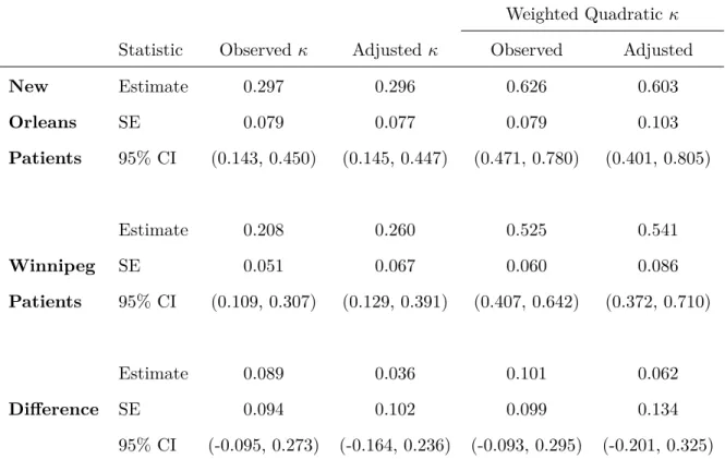
Table 1.8: Observed and adjusted estimates of agreement, corresponding standard errors and 0.95 confidence intervals.

New Estimate 0.297 0.296 0.626 0.603

Orleans SE 0.079 0.077 0.079 0.103

Patients 95% CI (0.143, 0.450) (0.145, 0.447) (0.471, 0.780) (0.401, 0.805)

Estimate 0.208 0.260 0.525 0.541

Winnipeg SE 0.051 0.067 0.060 0.086

Patients 95% CI (0.109, 0.307) (0.129, 0.391) (0.407, 0.642) (0.372, 0.710)

Estimate 0.089 0.036 0.101 0.062

Difference SE 0.094 0.102 0.099 0.134

95% CI (-0.095, 0.273) (-0.164, 0.236) (-0.093, 0.295) (-0.201, 0.325)

As shown in Table 1.8, there is better agreement for the New Orleans patients, since observer differences were mainly by only one category. Accordingly, the quadratic-weighted measures are larger than Kappa. For the Winnipeg patients, disagreements by two or more categories occurred more frequently than for the New Orleans patients, through the Winnipeg neurologist assigning categories 1 or 2 to patients assigned 3 or 4 by the New Orleans neurologist. Relative to the New Orleans patients, the agreement for the Winnipeg patients is to a somewhat larger extent better with the weighted adjusted methods than the adjusted Kappa, perhaps because the subgroup of Winnipeg patients had larger differences in the margins. On the other hand, the estimates in Table 1.8 suggest that the weighted kappa measures within both patient groups exhibit similar increasing trends. Since the estimated variances of the kappa statistics are larger for the New Orleans patient group (due to the smaller sample size), the agreement patterns may indeed be relatively similar in both patient groups.

(31)

in situ of the uterine cervix, seven pathologists were requested to evaluate and classify 118 slides separately into one of the following five categories based on the most involved lesion: (1) Negative; (2) Atypical Squamous Hyperplasia; (3) Carcinoma in Situ; (4) Squamous Carcinoma with Early Stromal Invasion; (5) Invasive Carcinoma. The frequency distributions from these diagnoses are presented in Table 1.9. In view of the substantial differences reflected in the marginal distributions shown in Table 1.9, the agreement among the pathologists on the classification of individual slides into the same category using the five-point scale is not expected to be very high. The diagnostic criteria for the five-point scale are not sufficiently precise to ensure a high level of inter-observer agreement. Consequently, a simplification in the scale is investigated by creating two classes by pooling diagnostic categories (1) and (2) versus combining (3),(4) and (5). This dichotomous classification is of clinical importance, as benign versus malignant lesions.

Table 1.9: Frequency distributions of diagnostic categories of the slides from uterine cervix by seven pathologists using Five-Point or Two-Point ordinal scale.

Pathologists

Scale A B C D E F G

(1) 26 27 31 38 16 62 32

(2) 26 12 42 48 31 31 20

(3) 38 69 37 23 53 20 61

(4) 22 7 6 8 14 1 3

(5) 6 3 2 1 4 4 2

(1) or (2) 52 39 73 86 47 93 52

(3) or (4) or (5) 66 79 45 32 71 25 66

* Diagnostic categories: (1) negative; (2) atypical squamous hyperplasia; (3) carcinoma in situ; (4) squamous

carcinoma with early stromal invasion; (5) invasive carcinoma.

(32)

(33)

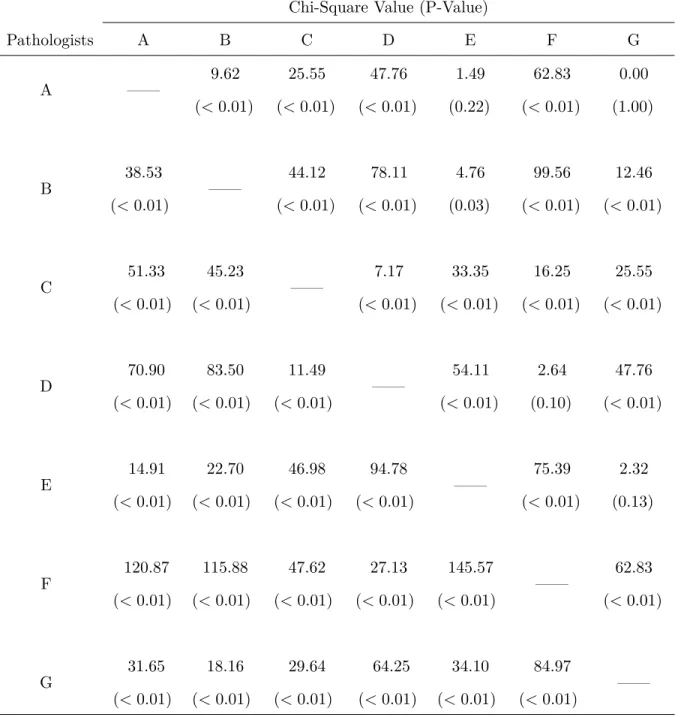
Table 1.10: Statistical tests of marginal homogeneity using Dichotomous scale(with D.F.=1) and Four-Point scale(with D.F.=3) between pairwise pathologists.

Chi-Square Value (P-Value)

Pathologists A B C D E F G

A —— 9.62 (<0.01) 25.55 (<0.01) 47.76 (<0.01) 1.49 (0.22) 62.83 (<0.01) 0.00 (1.00) B 38.53 (<0.01) —— 44.12 (<0.01) 78.11 (<0.01) 4.76 (0.03) 99.56 (<0.01) 12.46 (<0.01) C 51.33 (<0.01) 45.23 (<0.01) —— 7.17 (<0.01) 33.35 (<0.01) 16.25 (<0.01) 25.55 (<0.01) D 70.90 (<0.01) 83.50 (<0.01) 11.49 (<0.01) —— 54.11 (<0.01) 2.64 (0.10) 47.76 (<0.01) E 14.91 (<0.01) 22.70 (<0.01) 46.98 (<0.01) 94.78 (<0.01) —— 75.39 (<0.01) 2.32 (0.13) F 120.87 (<0.01) 115.88 (<0.01) 47.62 (<0.01) 27.13 (<0.01) 145.57 (<0.01) —— 62.83 (<0.01) G 31.65 (<0.01) 18.16 (<0.01) 29.64 (<0.01) 64.25 (<0.01) 34.10 (<0.01) 84.97 (<0.01) ——

* We combined diagnostic categories (4) and (5) together to produce the Four-Point scale. Results using

Dichotomous scale are above the diagonal, and Four-Point scale results are below the diagonal.

(34)

(35)

Table 1.11: Ordinary and adjusted Kappa (Standard Error) for pairs of pathologists using Dichoto-mous scale via El-Khorazaty formula.

Pathologists A B C D E F G

A —— 0.665 (0.069) 0.654 (0.064) 0.453 (0.066) 0.705 (0.066) 0.350 (0.062) 0.794 (0.056) B 0.727 (0.076) —— 0.435 (0.067) 0.310 (0.057) 0.745 (0.063) 0.234 (0.049) 0.735 (0.062) C 0.874 (0.087) 0.700 (0.113) —— 0.525 (0.081) 0.580 (0.066) 0.450 (0.082) 0.654 (0.064) D 0.817 (0.123) 0.760 (0.157) 0.580 (0.087) —— 0.364 (0.064) 0.563 (0.088) 0.453 (0.066) E 0.706 (0.069) 0.775 (0.066) 0.854 (0.100) 0.662 (0.125) —— 0.302 (0.058) 0.809 (0.055) F 0.778 (0.146) 0.717 (0.180) 0.573 (0.099) 0.618 (0.086) 0.757 (0.159) —— 0.350 (0.062) G 0.782 (0.059) 0.830 (0.071) 0.874 (0.087) 0.817 (0.123) 0.814 (0.058) 0.778 (0.146) ——

* Ordinary Kappa (SE) is above the diagonal; Adjusted Kappa (SE) is below the diagonal.

(36)

equation ( ˆψ−1)ˆπ2−ψˆˆπ+ 0.25 ˆψ= 0, we obtain ˆπ= √ ˆ ψ 2( √ ˆ

ψ+1). Therefore, the value of agreement Kappa is calculated as ˆκ = 2ˆ₁π₋−₀0_..₅5 =

2 √ ˆ ψ 2( √ ˆ

ψ+1)−0.5

0.5 =

√

ˆ

ψ−1

√

ˆ

ψ+1. We also derived the corresponding standard error for adjusted Kappa using Taylor series expansion, SE(ˆκ) = √ SE( ˆψ)

ˆ

ψ(

√

ˆ

ψ+1)2, where

model-based SE( ˆψ) = ˆψq_n2_ˆ_π +_n₍₀_.2₅₋_ˆ_π₎. For this particular example, the anticipated value of agreement Kappa between pathologists A and B from uniformly adjusted odds ratio is 0.727, which is the adjusted Kappa shown in Table 1.11; and the corresponding calculated standard error of Kappa is 0.063, which is close to the value presented in Table 1.11 as well. The numerical results indicate how well the adjusted Kappa reflects agreement independent of the observed margins with respect to the odds ratio. In fact, because of its stability across different margins, such interpretation is more appropriate with the adjusted Kappa than with the ordinary Kappa.

Table 1.12: Uniformly distributed proportions in agreement for binary classifications.

Rater B

Yes No Total

Rater A Yes π 0.5−π 0.5

No 0.5−π π 0.5

Total 0.5 0.5 1

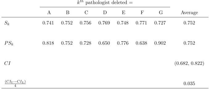
We also obtained the Jackknife confidence interval (CI) for the average adjusted pairwise Kappas shown in Table 1.13. For the average of 21 adjusted pairwise Kappas S, the kth pseudo-value P Sk with omission of the kth pathologist is calculated as P Sk = N S−(N −1)Sk, where Sk is

the average of 15 pairwise Kappas with excluding those with the kth observer. The jackknife CI was then calculated as CIJ(95%) =P S±2

q var

N , where var =

1

N−1

PN

k=1(P Sk−P S)2 , and

P S= _N1 PN_k₌₁P Sk = 0.752 =S. For this particular example, N = 7, and the Jackknife confidence

(37)

Table 1.13: Jackknife confidence interval (CI) for average adjusted pairwise Kappas.

kth pathologist deleted =

A B C D E F G Average

Sk 0.741 0.752 0.756 0.769 0.748 0.771 0.727 0.752

P Sk 0.818 0.752 0.728 0.650 0.776 0.638 0.902 0.752

CI (0.682, 0.822)

(CIU−CIL)

(38)

CHAPTER 2: OBSERVER VARIABILITY ANALYSIS WITH STANDARDIZATION FOR SUBJECT VARIABILITY

2.1 Overview

Usually, in any agreement study, observers (raters or interviewers) on different skill levels can be an important source of measurement error. When the data arising from such studies are quantitative, measures of inter-observer agreement are usually calculated as Introclass Correlation Coefficients (ICC) from Analysis of Variance (ANOVA). On the other hand, many observer reliability studies involve categorical data in which the response variable is classified into nominal (or ordinal) multinomial categories. Ordinary Kappa or weighted Kappa statistics have been recommended for the assessment of observer variability in these cases. In this paper, we propose an approach to the evaluation of observer agreement for categorical data by standardizing the raters’ classifications which reflect the extent to which the observers agree among themselves from underlying multidimensional contingency tables. We emphasize the adjusted quadratic-weighted pairwise Kappa statistics, which are comparable to the ICC, for the relevant assessments concerning inter-observer bias in the overall usage of the measurement scale and inter-observer agreement on the classification of individual subjects. For illustrative purposes, this general methodology is developed within the context of both simulated data structures and illustrative sets of a real clinical data.

2.2 Methods

2.2.1 Iterative Proportional Fitting (IPF) Algorithm

(39)

specified marginal row total distribution, and each column is proportionally adjusted to have its total equal the specified marginal column total distribution. This process is repeated iteratively until a specified level of convergence is reached.

2.2.2 Intraclass Correlation Coefficients (ICC)

The measuring of agreement between/among observations addresses the between/among variance expressed as a proportion of the total variance of the observations (i.e., the proportion of the total variability in the observations that is due to the differences between/among subjects). The ICCs, which relate the measurement error to the variability between subjects, are represented by the formula (A.2.4): ˆρI = ˆσ

2

s

ˆ

σ2

s+ˆσ2b+ˆσ2e =

n(M SS−M SE)

nM SS+rM SR+(nr−n−r)M SE. The variance component (σs2) represents the

variability among subjects, andσ2_b represents the variance due to systematic differences between raters. Theσ2

e is the residual variance. However, if one is only interested in the ranking of subjects,

the systematic differences between the raters are not important, and so ICC can be calculated as ˆ

ρI = σˆ 2

s

ˆ

σ2

s+ˆσ2e, ignoring systematic differences. Both types of ICCs are dependent on the heterogeneity of the population sample with respect to the observations in the study.

2.2.3 Quadratic Weighted Kappa

Some patterns of disagreement between the raters on the diagnostic classification of individual subjects can be investigated by specifying quadratic weights, wQ,ij = 1− (i−j)

2

(m−1)2; these weights

successively assign partial credits to the off-diagonal cells in order to create potentially less stringent reliability measures. In particular, quadratic-weighted Kappa is ICC’s counterpart, so that smaller disagreement patterns are more tolerated in the corresponding estimates of agreement. After adjustment to more clinically distributed marginal totals, the adjusted quadratic weighted Kappa statistics for the agreement between two raters can be expressed in the formulation κ∗_QW,jj0 =

[1−PL k=0

PL k0=0

(k−k0)2

L2 ]P

∗

jj0,kk0−[1−

PL k=0

PL k0=0

(k−k0)2

L2 ]P∗kP∗k0

1−[1−PL k=0

PL k0=0

(k−k0)2

L2 ]P∗kP∗k0

= 1− M SE ∗

jj0

PL k=0(k−¯y)

2_P

∗k

= ρ∗_I,jj0 (A.2.15) in

Appendix 2.5.1.

2.3 Examples

(40)

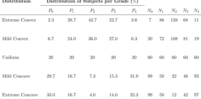
multiple raters is used to assess the distribution of the subjects across the 5 grades of the 5 scales. The distributions of master grades are described in Table 2.1 and randomly invoked disagreements are described in Table 2.2 (Mehta et al., 2018). In the simulation setup, the number of subjects chosen from each grade is fixed. This suggests some control of the random component involved when defining the population structure of the subjects. In general, differences from the master grade represent rater and scale quality. Ideally, these disagreements from the master grade would be low. High disagreements imply that the scale is unable to properly capture the true measurement and differentiate the grades or that the raters are poorly trained in the use of the scale. Table 2.2 (Mehta et al., 2018) shows the different levels of disagreement for the eight raters considered in the simulation scenarios. Case 1 through case 6 depict varying extents of rater disagreement ranging from acceptable to extreme disagreement. It should be noted that for each of the simulations, a random invocation of disagreements, as presented in Table 2.2, is performed on a set of subjects generated from a fixed distribution of master scores as shown in Table 2.1 (Mehta et al., 2018).

Simulation results in Table 2.3 (Mehta et al., 2018) suggest that for a fixed number of subjects (i.e., N=300), ICC from the convex distribution is smaller than ICC for the uniform distribution, which in turn is smaller than ICC for the concave distribution. The variance component estimates also show that the dissimilarity of ICC among distributions is attributed to the study design (i.e., distribution of subjects) as it corresponds to the variance component for subject variability, and not the scale quality variance component of rater error variability. The dependency of ICC on the distribution of subjects makes it difficult to compare results across reliability studies. This issue is addressed by Mehta et al. through a sampling method, that is proposed to reduce the nonuniformity, in the absence of a uniform distribution. To facilitate this investigation, data sets were simulated for each level of disagreement under extreme and mild concave and convex distributions with N = 300 subjects. The mean, median, and mode based on 8 ratings were calculated for each subject, and these statistics were then used to classify each subject into a unique grade. Samples of size n = 80 were then drawn.

(41)

samples based on all 3 methods are higher but closer to those for uniform data sets with N = 300. Specifically, the mode provided the smallest absolute difference from the uniform distribution across all 6 levels of disagreement. The same behavior is observed for mild concave cases. For extreme convex distributions, Table 2.3 illustrates that the samples based on all 3 methods have higher ICC values compared with the population due to reduction in subject non-uniformity. Upon sampling, ICC estimates are closer, but somewhat lower, relative to the standard uniform paradigm for low levels of disagreement. However, although sampling based on the mean produces estimates that are higher than the uniform distribution, as the levels of disagreement increase, the interpretation would be comparable. Hence, it follows that an unreliable scale is not made to appear reliable by the sampling procedure. Similar trends are observed for the mild convex distribution.

Table 2.1: Distribution of master grades with N=300

*This table is adapted from Mehta’s paper (Mehta et al., 2018)

Distribution Distribution of Subjects per Grade (%)

P0 P1 P2 P3 P4 N0 N1 N2 N3 N4

Extreme Convex 2.3 28.7 42.7 22.7 3.6 7 86 128 68 11

Mild Convex 6.7 24.0 36.0 27.0 6.3 20 72 108 81 19

Uniform 20 20 20 20 20 60 60 60 60 60

Mild Concave 29.7 16.7 7.3 15.3 31.0 89 50 22 46 93

Extreme Concave 33.0 16.7 4.0 14.0 32.3 99 50 12 42 97

(42)

Table 2.2: Cases pertaining to different levels of disagreement

Case Nature of Disagreement

1 20% subjects with 1-point disagreement for all raters (k=8)

2 20% subjects with 1-point disagreement for 75% of the raters (k=6)

30% with 1-point and 20% with 2-point disagreement for 25% of the raters (k=2)

5 20% subjects with 1-point disagreement, 10% with 2-point disagreement, 5% with 3-point disagreement and 5% with 4-point difference for 50% of the raters (k=4) 10% subjects with 1-point disagreement, 10% with 2-point disagreement, 10% with 3-point disagreement and 10% with 4-point difference for 50% of the raters (k=4)

(43)

Table 2.3: Mean ICC (and interdecile range) across 10000 simulations of uniform, convex and concave distributions with N=300 and samples of at least size n=80 form extreme and mild concave and convex distributions

Distri- Specifi- Levels of Disagreement

bution cations Case 1 Case 2 Case 3 Case 4 Case 5 Case 6

Extreme Full N=300 0.78(0.02) 0.58(0.04) 0.43(0.04) 0.30(0.04) 0.22(0.06) 0.08(0.04)

Convex Samp- Mean 0.86(0.02) 0.72(0.04) 0.58(0.06) 0.47(0.08) 0.39(0.09) 0.25(0.08)

ling Median 0.86(0.02) 0.72(0.04) 0.59(0.06) 0.47(0.07) 0.32(0.10) 0.16(0.08)

Mode 0.86(0.02) 0.72(0.04) 0.59(0.06) 0.46(0.07) 0.30(0.10) 0.14(0.08)

Mild Full N=300 0.82(0.02) 0.65(0.03) 0.51(0.04) 0.39(0.04) 0.26(0.06) 0.11(0.04)

Convex Samp- Mean 0.90(0.01) 0.80(0.03) 0.69(0.06) 0.57(0.08) 0.43(0.10) 0.27(0.08)

ling Median 0.90(0.01) 0.80(0.03) 0.70(0.04) 0.59(0.07) 0.39(0.10) 0.20(0.09)

Mode 0.90(0.01) 0.79(0.03) 0.68(0.05) 0.58(0.06) 0.36(0.09) 0.18(0.09)

Uniform Full N=300 0.90(0.01) 0.79(0.02) 0.68(0.03) 0.58(0.03) 0.34(0.05) 0.16(0.04)

Mild Full N=300 0.93(0.01) 0.84(0.02) 0.76(0.02) 0.69(0.03) 0.38(0.05) 0.19(0.04)

Concave Samp- Mean 0.90(0.01) 0.81(0.02) 0.75(0.02) 0.72(0.02) 0.56(0.07) 0.31(0.09)

ling Median 0.90(0.01) 0.80(0.02) 0.71(0.03) 0.65(0.03) 0.36(0.05) 0.28(0.08)

Mode 0.90(0.01) 0.80(0.02) 0.70(0.03) 0.61(0.03) 0.34(0.05) 0.18(0.05)

Extreme Full N=300 0.93(0.01) 0.85(0.02) 0.77(0.02) 0.69(0.02) 0.39(0.05) 0.19(0.04)

Concave Samp- Mean 0.91(0.01) 0.81(0.03) 0.75(0.02) 0.72(0.02) 0.56(0.07) 0.31(0.10)

ling Median 0.91(0.01) 0.81(0.03) 0.72(0.03) 0.65(0.03) 0.36(0.05) 0.28(0.08)

Mode 0.91(0.01) 0.81(0.02) 0.71(0.03) 0.63(0.03) 0.35(0.05) 0.18(0.04)

* Samples of size at least size n=80 were selected using the sampling method.

For assessment of agreement, the recent paper by Mehta (Mehta et al., 2018) focuses on how the intraclass correlation (ICC) depends on both distributions types, and on the nature of disagreement. For certain distributions, like convex distributions, the intraclass correlation will show lower agreement, even when the departure from the agreement is not strong. Mehta proposed standardization of the distribution so as to facilitate the assessment of different scales in populations with different distributions. Their paper used a sampling method, which has the limitation of not using all of the data, but it did enable standardization that provided a structure for agreement that was less dependent on the distribution, and thereby mainly dependent on the nature of the disagreement. Their sampling method also did not seem to have a way of generating confidence intervals, except perhaps via bootstrap re-sampling.

(44)

to the intraclass correlation results in Table 2.4. The average pairwise adjusted quadratic weighted Kappa estimates are in Table 2.6, and they are somewhat higher than the ICC ’s from the sampling method for the mild convex distribution and the extreme convex distributions. Therefore, the application of the adjusted quadratic weighted Kappa can address different types of distributions and different patterns of departures.

Table 2.4: Intraclass Correlation (ICC) of ratings on the same subject (Subjects=300, Raters=8)

Distribution Case 1 Case 2 Case 3 Case 4 Case 5 Case 6

Extreme Concave 0.932 0.861 0.771 0.685 0.391 0.175

Mild Concave 0.928 0.852 0.758 0.668 0.375 0.172

Uniform 0.900 0.801 0.677 0.571 0.339 0.147

Mild Convex 0.824 0.679 0.511 0.375 0.248 0.121

Extreme Convex 0.779 0.606 0.429 0.296 0.197 0.104

Table 2.5: Average pairwise quadratic weighted Kappa (Subjects=300, Raters=8)

Distribution Case 1 Case 2 Case 3 Case 4 Case 5 Case 6 Extreme Concave 0.932 0.855 0.759 0.676 0.390 0.175

Mild Concave 0.928 0.845 0.746 0.660 0.374 0.172

Uniform 0.900 0.797 0.669 0.565 0.338 0.147

Mild Convex 0.824 0.691 0.520 0.380 0.247 0.123