Methods and Approaches for Evaluating the Validity of
Latent Class Models with Applications
Marcus Berzofsky
A dissertation submitted to the faculty of the University of North Carolina at Chapel Hill in partial fulfillment of the requirements for the degree of Doctor of Public Health in the School of Public Health (Biostatistics).
Chapel Hill 2011
Approved by:
Paul Biemer
William Kalsbeek
Amy Herring
Chris Wiesen
ABSTRACT
MARCUS BERZOFSKY: Methods and Approaches for Evaluating the Validity of Latent Class Models with Applications
(Under the direction of Paul Biemer and William Kalsbeek)
This dissertation focuses on methods for assessing classification error for sensitive,
categorical outcomes by using latent class analysis (LCA) and Markov latent class analysis
(MLCA). The ability to quantify classification error in a survey is critical to understanding
the quality of its estimates. Classification error (measurement error for categorical outcomes)
is defined as the difference between the true value of a measurement and the value obtained
during the measurement process. For dichotomous outcomes there are two types of
classification errors: a false positive (i.e., response is affirmative when the negative is
correct) and a false negative (i.e., response is negative when the affirmative is correct). A
sensitive outcome is an event for which respondents have a negligible probability of
providing false positive responses. Such events are very important in the study of socially
undesirable phenomenon (e.g., alcohol abuse, sexual misconduct, or drug abuse). LCA, for
cross-sectional data, and MLCA, for panel or longitudinal data, are modeling techniques that
use repeated measurements rather than an error-free estimate to estimate the true prevalence
of an outcome and its corresponding classification error.
The dissertation is split into three parts. First, I assess the impact of local dependence,
the key assumption in LCA, on classification error estimates. I use simulation to determine
the impact of local dependence. Then, I develop an approach to correct for local dependence
Second, I determine if there is a more parsimonious way to incorporate time varying
grouping variables (variables that do not change in a linear fashion over time) in an MLC
model. I develop a process to test time-invariant summary variables and determine if model
fit is not impacted. I then determine if time-invariant summary variables are appropriate for
the National Crime Victimization Survey (NCVS). Third, I estimate the classification error
rates for the NCVS. To achieve this, I develop a process to ensure that model estimates meet
all assumptions. I found that the NCVS has a large amount of classification error and
ACKNOWLEDGMENTS
This dissertation would not have been possible without the love and support of so
many people. My wife, Jessica, whose encouragement helped me see this process to the end.
My children, Curtis and Claudia, who were not even born when I started this journey,
inspired me to finish. And, my advisors, Paul Biemer and Bill Kalsbeek, whose patience and
TABLE OF CONTENTS
LIST OF TABLES ... ix
LIST OF FIGURES ... xi
Chapter 1. Introduction ...1
1.1 Motivation for Quantifying Measurement Error in Surveys ...1
1.1.1 Defining Measurement Error ...1
1.1.2 Classification Error and Its Importance ...2
1.2 Current Approaches for Estimating Measurement Error ...5
1.2.1 Approaches ...5
1.3 Topics of this Dissertation ...10
1.4 References...13
2. Modeling Local Dependence in a Latent Class Analysis of Sensitive Questions ...16
2.1 Chapter Summary ...16
2.2 Introduction...16
2.2.1 Motivation ...19
2.3 Simulations ...25
2.3.1 Bivocality ...25
2.3.2 Correlated Error ...27
2.3.3 Group Heterogeneity ...29
2.4 Diagnostic Procedures for Testing and Correcting Local
Dependence...33
2.5 A General Approach to Diagnosing and Correcting LCM with Three Indicators ...34
2.6 Application ...37
2.7 The Five-Indicator Model ...38
2.8 Testing of Diagnostic Procedures on Three-Indicator Models ...40
2.9 Discussion ...43
2.10 Conclusions ...45
2.11 References...47
3. Time Varying Grouping Variables in Markov Latent Class Analysis: Some Problems and Solutions ...49
3.1 Chapter Summary ...49
3.2 Introduction...50
3.3 Methods ...57
3.4 Analysis ...64
3.4.1 Overview of the NCVS ...64
3.4.2 Development of Alternative Models ...67
3.5 Results ...73
3.5.1 Results of Comparisons of Time-invariant Summary Models ...73
3.5.2 Results of Comparisons of Reduced Time Varying Grouping Variable Models ...76
3.5.3 Comparison of the Best Time-invariant Summary Models and the Best Time Varying Models ...79
3.5.4 Discussion ...83
3.6 Analysis of the Measurement Error and Prevalence Estimates ...84
3.8 References...90
4. Quantifying Classification Error in the National Crime Victimization Survey: A Markov Latent Class Analysis ...92
4.1 Chapter Summary ...92
4.2 Background ...93
4.3 Purpose ...98
4.4 Methods ...101
4.4.1 Technical Description of MLCA and Its Assumptions...101
4.4.2 The Data, Outcomes, and Grouping Variables ...105
4.4.3 Model Selection ...107
4.4.4 Other Analyses ...112
4.5 Analysis ...114
4.6 Results ...116
4.7 Discussion ...121
4.7.1 High False Negative Rates in the NCVS ...121
4.7.2 Decreasing Prevalence Rates over Time ...123
4.7.3 Classification Error among Demographic Groups ...124
4.7.4 Implications to Published NCVS Estimates ...125
4.7.5 Limitations ...125
4.8 Conclusions ...126
LIST OF TABLES
Table
2.1 Definition of NIS LCA Indicators for Inmate-on-Inmate
Sexual Victimization...22
2.2 NIS Unadjusted Three-Indicator LCM ...24
2.3 Assumptions Used in Expeculation of Group Heterogeneity ...31
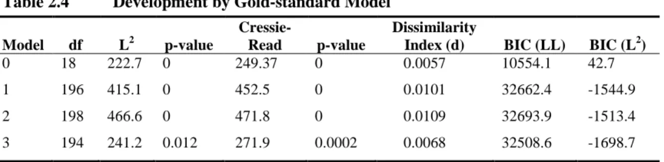
2.4 Development by Gold-standard Model...39
2.5 Parameter Estimates from the Gold-standard Model ...40
2.6 Frequency of Statistically Similar Parameter Estimates by Model Type ...42
2.7 Frequency of Parameter Estimates with a Smaller Absolute Bias after Applying Corrective Procedures ...43
3.1 Classification Error and Prevalence Estimates1 from the Population Model, by Type of Crime Victimization and Grouping Variable ...73
3.2 Fit Statistics for Time-Invariant Summary Models, by Type of Crime Victimization and Grouping Variable...74
3.3 Bias in Estimates Between Time-Invariant Summary Variable Recode Models and the Population Model, by Type of Crime Victimization and Grouping Variable Based on Synthetic Data ...75
3.4 Fit Statistics for Reduced Time Varying Grouping Variable Models, by Type of Crime Victimization and Grouping Variable ...77
3.5 Bias in Estimates between Reduced Time Varying Grouping Variable Models and the Population Model, by Type of Crime Victimization and Grouping Variable Based on Synthetic Data ...78
3.6 Percentage of Table Cells with Five or Fewer Observations, by Time Varying Grouping Variable and Model Data Table ...81
3.7 Classification Error and Prevalence Estimates from Best Time-invariant Summary and Time Varying Grouping Variable Models Based on Actual NCVS Data...83
4.1 Illustration of Decreasing Trend in Crime Victimization Rates without Any Classification Error ...100
4.3 Fit Statistics for Crimes against a Household Models by Set of Waves
Included ...116
4.4 Classification Errors by Wave and Set of Waves Modeled for Less
Serious Crimes against an Individual ...118
4.5 Classification Errors by Wave and Set of Waves Modeled for Crimes
against a Household ...118
4.6 Evidence Rating of Classification Error Differences for Demographic
Variables ...119
4.7 Average Classification Error Rates for Demographic Variables with a
Strong Evidence Rating ...120
LIST OF FIGURES
Figure
2.1 Path diagram for LC model with three indicators and no grouping
variables. ...19
2.2 Relative bias in the false negative rate of a bivocal indicator by
correlation level between the latent variables X and Y. ...27
2.3 Relative Bias in Estimated Prevalence Probability due to Correlated
Error as a Function of the Correlation and False Negative Probability ...29
2.4 False negative rate in indicator by group as correlation between G and H
increases. ...32
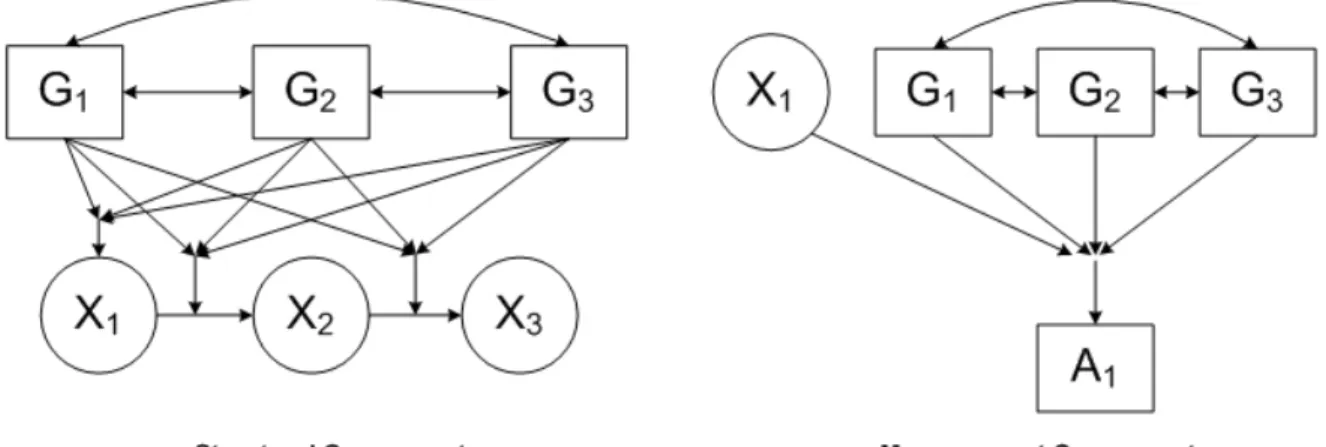
3.1 Path diagram for MLC model with three time points and no grouping variables, with a measurement component that assume
time-homogeneous classification errors (i.e., A1|X1=A2|X2=A3|X3). ...53
3.2 Path diagram for the population model that assumes time-homogeneous classification (i.e., A1|X1G1G2G3= A2|X2G1G2G3= A3|X3G1G2G3). Double arrows indicate a three-way interaction (i.e., G1G2G3). The figure only shows the path diagram for the measurement component of indicator A1. The diagram for the measurement component is similar for the other two
indicators: A2|X2G1G2G3 and A3|X3G1G2G3. ...59 3.3 Path diagram for models with time-invariant summary grouping
variables that assume time-homogeneous classification errors (i.e.,
A1|X1G= A2|X2G= A3|X3G). ...68 3.4 Path diagram for M(R1) that assumes time-homogeneous classification
errors (i.e., A1|X1 G1= A2|X2G2= A3|X3G3.). Double arrows indicate a
three-way interaction (i.e., G1G2G3). ...71 3.5 Path diagram for M(R2) that assumes time-homogeneous classification
(i.e., A1|X1G1G2G3= A2|X2G1G2G3= A3|X3G1G2G3). Double arrows indicate a three-way interaction (i.e., G1G2G3). The figure only shows the path diagram for the measurement component of indicator A1. The diagram for the measurement component is similar for the other two
indicators: A2|X2G1G2G3 and A3|X3G1G2G3. ...72 4.1 Path diagram for model MLC model with grouping variable that
assumes time-homogeneous classification errors (i.e., A1|X1G= A2|X2G=
1. Introduction
1.1 Motivation for Quantifying Measurement Error in Surveys 1.1.1 Defining Measurement Error
Measurement error is defined as the difference between the true value of a
measurement and the value obtained during the measurement process (Biemer, 2011; Lessler
& Kalsbeek, 1992). Sudman and Bradburn (1974) write that the conceptual framework of
measurement error comes from one of three sources: the task to be accomplished, the
interviewer, or the respondent. The task to be accomplished includes the mode of the
interview (e.g., in person or via telephone) and the questionnaire itself. In terms of the mode,
the nature of the interview (e.g., sensitive subject matter) may impact how a respondent
answers if they are talking directly to an interviewer as opposed to answering an unseen
person or, in the case of audio computer-assisted self-interviews (ACASI), a computer. The
questionnaire impacts measurement error by how it is structured. Sudman and Bradburn
indicate that measurement error will be smaller if the questionnaire has greater structure and
is laid out clearly. The second source of measurement error is the interviewer. Whether the
interviewer is required to follow a strict script or is allowed leeway in obtaining responses
impacts the level of measurement error. The third source of measurement error is the
respondent. Sudman and Bradburn state that the motivation of the respondent plays a major
role in the quality of the data provided.
As a type of nonsampling error, measurement error cannot be corrected for during the
impact of measurement error on survey estimates prior to drawing any conclusions. Lohr
(1999, pp. 9–10) outlines eight ways in which a measurement error may be induced that fit
into the Sudman and Bradburn framework:
• People sometimes do not tell the truth
• People do not always understand the questions
• People forget (e.g., telescoping or recall bias)
• People give different answers to different interviewers
• People may say what they think an interviewer wants to hear or what they think
will impress the interviewer
• A particular interviewer may affect the accuracy of the response by misreading
questions, recording responses inaccurately, or antagonizing the respondent
• Certain words mean different things to different people
• Question wording and order have a large effect on responses obtained.
1.1.2 Classification Error and Its Importance
The goal of many surveys today is to determine estimates for topics that are
considered sensitive in nature. These estimates are desired at both the national and
subpopulation level. Some examples of these types of surveys are the National Inmate
Survey (NIS), which estimates the prevalence of sexual victimization in correctional
facilities; the National Crime Victimization Survey (NCVS), which measures the prevalence
of all types of crime in the United States; the National Survey on Drug Use and Health
(NSDUH), which in addition to other factors, measures the use of legal and illegal drugs in
the United States; and the Current Population Survey (CPS), which among other things,
methodologists have developed methods to make the respondents feel more comfortable
taking the interview. For example, the NIS and NSDUH use ACASI, which allow
respondents to answer survey questions by using laptops. Therefore, respondents do not need
to tell the interviewer anything sensitive. Tools such as ACASI are believed to reduce bias in
survey estimates because studies have shown that they yield higher prevalence estimates for
sensitive subjects such as drug use (Turner et al., 1998; Epstein, Barker, & Kroutil, 2001),
but they do not completely ensure that a respondent is giving a truthful answer. This could be
because the respondent truly does not want anyone to know what he/she has done or what has
happened to him/her, or the respondent has simply forgotten because of a traumatic
experience or faulty memory.
Instances in which respondents are not classified correctly are called classification
errors. Particularly for surveys that attempt to quantify sensitive subject matter, the rate of
classification error can be quite high, and the need to quantify this error is important to
evaluate the quality of inferences based upon the survey estimates. Although measurement
error—and specifically classification error—can occur in all surveys regardless of the
sensitivity level of the topic, surveys dealing with sensitive topics offer special challenges
that require further research. For example, there are subpopulations that will always be
untruthful in a survey when asked about a sensitive topic. For instance, some people will
always deny using illicit drugs or participating in criminal activity regardless of how many
times they are asked.
For dichotomous items, classification error leads to false positives (answers in the
affirmative when negative answers are correct) and false negatives (answers in the negative
(1996) and Biemer and Bushery (2001) examined the CPS to determine how well it classified
respondents by employment status. Their results suggested that only 67.6% of truly
unemployed persons were classified correctly, while employed persons or persons not in the
labor force were almost always classified correctly. When considering sensitive subject
matter, this finding seems reasonable because a response of “unemployed” is probably the
most undesirable answer respondents could give, and therefore, it is the answer about which
respondents are most likely to be misleading. Furthermore, Biemer and Wiesen (2002)
looked into potential classification error in the NSDUH survey (called the National
Household Survey on Drug Abuse [NHSDA] during the survey years studied) regarding the
prevalence of past year marijuana use. The survey had three questions related to marijuana
use: two that asked about whether one was a “user” of marijuana and one that asked about
frequency of use. Their analysis showed that the questions asking if one was a user had a
much higher false negative rate than the frequency item. Further analysis found that 59% of
respondents who indicated that they were not users also indicated that they were infrequent
(i.e., 1 to 2 days in the past year) users of marijuana. In other words, many of those who tried
marijuana a couple times over the past year did not consider themselves users of marijuana
and, therefore, did not classify themselves as such.
Without measuring the classification error in the previous examples, analysts would
have underestimated the prevalence estimates they were trying to measure. This seems
reasonable because, in both the case of unemployment and drug use, respondents are more
likely to give false negative responses (i.e., to answer that they are employed or do not use
drugs when they are unemployed or do use drugs) rather than false positives (i.e., to answer
1.2 Current Approaches for Estimating Measurement Error 1.2.1 Approaches
To quantify measurement error in categorical variables, statisticians have usually
used one or more of four methods. Each of these methods quantifies measurement error in a
different way and uses different assumptions. The four methods and the way in which they
quantify measurement error are the following:
• Gold-standard method—directly measures bias between measurement with error
and an error-free measurement
• Reliability analysis—decomposes the variance to ascertain the portion of an
estimate’s variance that is due to measurement error
• Latent class analysis (LCA)—uses maximum likelihood estimation (MLE) to
create estimates free of measurement error and the corresponding classification
error rates to allow one to determine the bias between the survey estimates and the
MLE
• Markov latent class analysis (MLCA)—uses a similar approach to LCA, but is
designed for panel or longitudinal surveys.
Because each of these methods make different assumptions and use different
methods, they may lead to different conclusions. Therefore, using multiple methods acts as a
confirmatory process. A statistician may use one method as the main approach, but may also
use a second or third to verify the results. If the conclusions under each method are the same,
then one can have greater confidence that the conclusions under the main approach are
necessary to see why the two methods differ and, if possible, to determine which method
provided the erroneous result.
Gold Standard
The gold-standard method compares two measurements to directly calculate the bias
and classification error rates between the two methods. In the gold-standard method, the first
measurement is assumed to be fallible, or with error, and the second method is assumed to be
infallible, or without error. Bross (1954) and Tenenbein (1972) first demonstrated how one
can directly calculate the bias and classification error rates for the fallible measurement.
When a true gold standard exists, the gold-standard method provides the greatest
ability to accurately quantify measurement error. The gold-standard method is the only
method that provides direct estimates of the item of interest without measurement error.
Moreover, as Bross (1954) and later Tenenbein (1972) demonstrate, the false negative and
false positive rates and the resulting bias from a self-reported or otherwise fallible method
can be directly calculated when compared to the true value.
However, the disadvantage of the gold-standard method is that it rarely exists and, in
cases where one assumes it does, there may be latent (unobserved) error in the gold-standard
estimate, which could lead to invalid conclusions. For example, several studies have found
that reconciled data, used as the gold standard, can be erroneous (Biemer & Forsman, 1992;
Sinclair & Gastwirth, 1996; Biemer, Woltman, Raglin, & Hill, 2001). For example, Biemer
and Forsman (1992) found that in the CPS, up to 50% of the errors in the original interview
are not detected in the reconciled reinterview. Furthermore, the use of administrative records
as a gold standard can prove faulty because of differences in the reference period,
definitional differences, and missing or underreported data (Jay, Belli, & Lepkowski, 1994;
Moreover, the use of external tests for validation often have nonnegligible error rates,
even though it is usually assumed otherwise. For example, biological tests have been found
to have substantial false negative and false positive rates for certain types of drugs (Visher &
McFadden, 1991). Also, a study comparing medical diagnoses made by a computer to those
of a physician overestimated the number of errors made by the computer because it assumed
the physician’s diagnosis was always correct (Van Meerten, Durinck, & Dewit, 1971).
Reliability Analysis
Reliability analysis uses resampling theory to decompose an estimate’s variance into
two components: sampling variance and simple response variance. Sampling variance is the
variation due to the drawing of a simple random sample. Simple response variance is the
trial-to-trial variation among a respondent’s answers and represents the additional variation
due to measurement error. Hansen, Hurwitz, and Pritzker (1964) showed how the ratio of
simple random variance over the total variance can be used to assess the quality of an
estimate relative to its level of measurement error.
Reliability analysis allows analysts to measure the level of inconsistency in how a
respondent answers a particular item when no gold standard is available for comparison.
Using Census Bureau guidelines, this analysis allows for a simple measurement of how well
the item of interest is measuring the intended subject matter (U.S. Census Bureau, 1985).
When dealing with continuous outcomes, the reliability ratio has a very eloquent and
simple interpretation. For example, an observation can take the form yi =µi+εi, where yiis
the observed value, µiis the true value, and εiis the measurement error associated with the
observation. Under this scenario, the
( )
2 iVarµ =σµ and
( )
2 i
uncorrelated. Therefore, 2 2
2 R
ε µ
µ
σ + σ
σ
= is the reliability ratio that represents the proportion of
the total variance because of sampling error. However, dealing with a dichotomous outcome
and the sample proportion, this interpretation is not clear because the measurement error is
directly correlated to a person’s response. To illustrate this, using the formula yi =µi+εiif
1 i =
µ for person i, but yi =0, then εimust equal -1. Therefore, the interpretation of the
reliability ratio is not as clear.
Latent Class Analysis
LCA is a modeling approach for estimating the parameters of a categorical data table
subject to misclassification and was developed by Lazarsfeld and Henry (1968). The method
is related to finite mixture modeling (McLachlan & Peel, 2000) and log-linear modeling with
latent variables (Hagenaars, 1993). In LCA, the true survey characteristic is treated as an
unobservable (or latent) variable. Under some assumptions (e.g., local independence, group
homogeneity, Markov, and homogeneous classification error), which are described in detail
later in the dissertation, the missing latent variable can be estimated using MLE. Usually the
EM algorithm is used to provide estimates of the true population proportion and the
misclassification probabilities (Dempster, Laird, & Rubin, 1977). For survey methodologists,
LCA is an important tool for studying the measurement error (bias and variance) for survey
questions for situations in which there is no possibility of obtaining error-free values for the
characteristics of interest.
LCA has three critical advantages over other techniques for assessing measurement
error in survey estimates such as the gold-standard method (Bross, 1954; Tenenbein, 1972)
or reliability analysis (Hansen et al., 1964). First, unlike methods that rely on a gold standard,
for a dichotomous latent variable, LCA provides model-based estimates of the truth as well
as estimates of the false negative and false positive error probabilities (Biemer, 2004). Third,
in addition to assessing the quality of the survey estimates, LCA can assess the quality of the
questions being used to estimate the outcome of interest (Biemer & Wiesen, 2002; Kreuter,
Yan, & Tourangeau, 2008).
However, LCA also has a number of disadvantages (Biemer, 2011). For example,
LCA makes several strong assumptions be met for estimates to be valid. These assumptions
are often difficult to meet in a complex survey environment. Furthermore, LCA gives poor
results with sparse data (i.e., a large proportion of small or zero frequency cells in the data
table). Sparse data can cause problems with model identification, model selection, and
parameter estimation. Moreover, replicate measures may be difficult to obtain. It is often
difficult for survey designers to create multiple measures of the latent variable without
appearing redundant to the respondent.
Markov Latent Class Analysis
MLCA is analogous to LCA for panel or longitudinal surveys and was first proposed
by Wiggins (1973). Like LCA, MLCA treats a respondent’s true response as latent or
unknown because there is no way to verify the accuracy of the manifest variables, which are
measurement items in the survey that attempt to estimate the latent characteristic. Unlike
LCA, MLCA uses multiple time points to assess the accuracy of a person’s response. In other
words, MLCA requires only one manifest measurement at each time point to estimate the
latent variable at each time point and the classification error rates of the manifest variables.
Because of this feature, a minimum of three time points are required to conduct MLCA.
Furthermore, MLCA uses maximum likelihood to estimate the latent variables and the
MLCA offers several advantages for quantifying measurement error. Without the
availability of a gold standard, MLCA is the only method that incorporates the panel or
longitudinal design. In doing so, MLCA takes advantage of all the information provided by a
respondent over time (Biemer & Bushery, 2001). Furthermore, MLCA requires only one
measurement per time point, and it does not require reinterview data, which can save cost
and time (Tran & Winters, 2003). Moreover, Biemer and Bushery (2001) point out that
obtaining reinterview data in a panel study is often impractical. In addition, Biemer and
Bushery state that often reinterview data is only collected on a subset of the initial sample.
MLCA can use information from the entire panel data set.
However, like LCA, an MLCA requires several assumptions for its models to be
identifiable (e.g., first-order Markov, independent classification errors, homogeneous
classification errors, and time homogeneous errors). If these assumptions are violated, then
conclusions based on that model may be erroneous. For instance, in the CPS, Tran and
Winters (2003) hypothesize that the portion of the population that becomes unemployed and
stays unemployed for a long time could violate the Markov assumption. MLCA requires at
least three time points. Therefore, in settings other than a panel study or longitudinal study,
MLCA cannot be used.
1.3 Topics of this Dissertation
This dissertation focuses on using LCA and MLCA to quantify classification error in
surveys. The dissertation is split into three parts. Each part focuses on methods to assess the
LC model or MLC model to understand the implications of violations of key model
Chapter 2 looks at the key assumption in LCA: local independence. If local
independence is not met, then the model is locally dependent, which causes poor model fit,
creates bias in the parameter estimates, and makes the standard errors for the estimates too
large (Pepe & Janes, 2007; Sepulveda, Vicente-Villardon, & Galindo, 2008). The chapter
breaks local dependence into three possible sources: bivocality, correlated error, or latent
heterogeneity. Through simulation, the impact on parameter estimates is assessed for each
source of local dependence. Then, the chapter reviews the literature for approaches to correct
for local dependence when it occurs. Based on these approaches, I propose a process by
which one can check for local dependence and develop a model that corrects for any sources
of local dependence should they be identified. I then apply my proposed process to data from
the NIS to assess its ability to identify and correct for local dependence.
Chapter 3 looks at how best to use time varying grouping variables (i.e., variables that
change in nonlinear manner over time) in an MLC model. In a panel or longitudinal survey
some manifest variables (i.e., variables obtained during the survey interview) are time
varying because they change over time in a nonlinear fashion (e.g., mode of interview,
whether a person has health insurance). Variables that do not change over time are known as
time invariant grouping variables. Both time invariant and time varying grouping variables
are used in an MLC model to create homogeneity in the classification error rates. Although
time varying grouping variables provide more information for the model than a static
equivalent, they require a large number of model parameters, which use up the available
degrees of freedom and cause sparseness in the data that impact the model fit (Biemer &
Berzofsky 2011; Vermunt, Langeheine, & Bockenholt, 1999). This chapter determines if a
variable through a static variable) can provide as good of model fit as when the actual time
varying grouping variable is used. To do this, I develop a general approach for comparing
models using a time varying grouping variable to various types of time-invariant summary
variables. I use the NCVS as an empirical data set to test my proposed approach.
Chapter 4 conducts the first assessment of classification error in the NCVS. I use
MLCA to estimate the classification error rates. The chapter assesses the overall
classification error rates in the NCVS, whether the rates change over time, whether certain
demographic groups are more prone to classification error, and how the published NCVS
estimates would be impacted if classification error was accounted for in the estimate process.
In conducting the MLCA, I propose an approach that tests the model assumptions and
1.4 References
Bross, I. (1954). Misclassification in 2 X 2 tables. Biometrics, 10, 478–486.
Biemer, P. (2004). Simple response variance: then and now. Journal of Official Statistics, 20, 417–439.
Biemer, P. P. (2011). Latent Class Analysis of Survey Error. Hoboken, NJ: John Wiley & Sons.
Biemer, P., & Berzofsky, M. (2011). Some issues in the application of latent class models for questionnaire design. In J. Madans, K. Miller, G. Willis, & A. Maitland (Eds.).
Questionnaire evaluation methods, Hoboken, NJ: John Wiley & Sons.
Biemer, P., & Bushery, J. (2001). Application of Markov latent class analysis to the CPS.
Survey Methodology, 26(2), 136–152.
Biemer, P. P., & Forsman, G. (1992). On the quality of reinterview data with applications to the Current Population Survey. Journal of the American Statistical Association,
87(420), 915–923.
Biemer, P., & Wiesen, C. (2002). Latent class analysis of embedded repeated measurements: An application to the National Household Survey on Drug Abuse. Journal of the
Royal Statistical Society: Series A, 165(1), 97–119.
Biemer, P. P., Woltman, H., Raglin, D., & Hill, J. (2001). Enumeration accuracy in a population census: an evaluation using latent class analysis. Journal of Official
Statistics, 17(1), 129–149.
Dempster, A., Laird, N., & Rubin, D. (1977). Maximum likelihood from incomplete data via the EM algorithm. Journal of the Royal Statistical Society: Series B, 39(1), 1–38.
Epstein, J. F., Barker, P. R., & Kroutil, L. A. (2001). Mode effects in self-reported mental health data. Public Opinion Quarterly, 65(4), 529–549.
Hagenaars, J. A. (1993). Loglinear models with latent variables. Newbury Park, CA: Sage Publications.
Hansen, M., Hurwitz, W. N., & Pritzker, L. (1964). The estimation and interpretation of gross differences and the simple response variance. In C. R. Rao (Ed.), Contributions
to statistics (pp. 111–136). Calcutta: Pergamon Press, Ltd.
Jay, G., Belli, R., & Lepkowski, J. (1994). Quality of last doctor visit reports: a comparison of medical records and survey data. Proceedings of the ASA Section on Survey
Kreuter, F., Yan, T., & Tourangeau, R. (2008). Good item or bad—Can latent class analysis tell? The utility of latent class analysis for the evaluation of survey questions. Journal
of the Royal Statistical Society: Series A, 171(3), 723-738.
Lazarsfeld, P. F., & Henry, N. W. (1968). Latent structure analysis. Boston: Houghton Mifflin.
Lessler, J. T., & Kalsbeek, W. D. (1992). Nonsampling error in surveys. New York: Wiley.
Lohr, S. L. (1999). Sampling: Design and analysis. New York: Duxbury Press.
Marquis, K. (1978). Inferring health interview response bias from imperfect record checks.
Proceedings of the ASA Section on Survey Research Methods, 265–270.
McLachlan, G. J., & Peel, D. (2000). Finite mixture models. New York: Wiley.
Pepe, M. S., & Janes, H. (2007). Insights into latent class analysis of diagnostic test performance. Biostatistics, 8(2), 474−484.
Sinclair, M., & Gastwirth, J. (1996). On procedures for evaluating the effectiveness of reinterview survey methods: Application to labor force data. Journal of the American
Statistical Association, 91, 961–969.
Sudman, S., & Bradburn, N. M. (1974). Response effects in surveys: A review and synthesis. Chicago: Aldine.
Sepulveda, R., Vicente-Villardon, J. L., & Galindo, M. P. (2008). The biplot as a diagnostic tool of local dependence in latent class models. A medical application. Statistics in
Medicine, 27(11), 1855−1869.
Tenenbein, A. (1972). A double sampling scheme for estimating from misclassified
multinomial data with application to sampling inspection. Technometrics, 14(1), 187– 202.
Tran, B., & Winters, F. (2003). Markov latent class analysis and its application to the Current Population Survey in estimation response error. Proceedings of the 2003 Joint
Statistics Meeting Section on Survey Research, 4267–4273.
Turner, C. F., Ku, L., Rogers, S. M., Lindberg, L. D., Pleck, J. H., & Sonenstein, F. L. (1998). Adolescent sexual behavior, drug use, and violence: Increased reporting with computer survey technology. Science, 280(5365), 867–873.
U.S. Census Bureau. (1985). Evaluating censuses of population and housing (STD-ISP-TR-5). Washington, DC: U.S. Government Printing Office.
Vermunt, J. K., Langeheine, R., & Bockenholt, U. (1999). Discrete-time discrete-state latent Markov models with time-constant and time-varying covariates. Journal of
Educational and Behavioral Statistics, 24(2), 179-207.
Visher, C. A., & McFadden, K. (1991). A comparison of urinalysis technologies for drug
testing in criminal justice. National Institute of Justice Research in Action.
Washington, DC: U.S. Department of Justice.
Wiggins, L. M. (1973). Panel analysis, latent probability models for attitude and behavior
2. Modeling Local Dependence in a Latent Class Analysis of Sensitive Questions 2.1 Chapter Summary
Latent class analysis (LCA) is a powerful tool in surveys to assess the quality of an
estimate and the classification error rates associated with a particular survey item when no
gold-standard estimate is available. LCA’s main assumption is local dependence. This
chapter divides local dependence into its three key components: bivocality, correlated error,
and heterogeneity. Each component is then assessed to see how it affects estimates from a
latent class model (LCM). Focusing on surveys targeting sensitive outcomes, I propose a
theoretical framework by which each aspect of local dependence can be diagnosed and
corrected. I empirically tested the proposed framework for three-indicator models using data
from the 2007 National Inmate Survey (NIS), finding that the proposed framework mitigated
some, but not all, of the local dependence regardless of which aspects of local dependence
were present. The framework performed best when there were no bivocal indicators present
in the model.
2.2 Introduction
The assessment and reduction of measurement error in surveys is a growing area of
research. Measurement error is the difference between the true value of a measurement and
the value obtained during the measurement process (Lessler & Kalsbeek, 1992). Some
techniques for reducing measurement error can be used during the interview, such as
interviewing techniques, like audio computer-assisted self-interviewing (ACASI), which
& Kroutil, 2001; Turner et al., 1998), but do not completely ensure that respondents give
truthful answers. Therefore, most techniques to assess the quality of a survey estimate are
conducted after data collection is complete. One such technique is LCA (Lazarsfeld &
Henry, 1968). Although LCA is more than 50 years old, it has only recently been used to
improve the quality of surveys (Biemer, 2004).
LCA has three critical advantages over other techniques for assessing measurement
error in survey estimates, such as the gold-standard method (Bross, 1954; Tenenbein, 1972)
or reliability analysis (Hansen, Hurwitz, & Pritzker, 1964). First, unlike methods that rely on
a gold standard, LCA does not require the assumption that any of the measurements are error
free. Second, for a dichotomous latent variable, LCA provides model-based estimates of the
truth as well as estimates of the false negative and false positive error probabilities (Biemer,
2004). Third, in addition to assessing the quality of the survey estimates, LCA can assess the
quality of the questions being used to estimate the outcome of interest (Biemer & Wiesen,
2002; Kreuter, Yan, & Tourangeau, 2008).
LCA also has a number of disadvantages and criticisms (Biemer, 2011). For example,
LCA makes strong assumptions, like requiring several assumptions be met for estimates to be
valid. These assumptions are often difficult to meet in a complex survey environment.
Furthermore, LCA gives poor results with sparse data (i.e., a large proportion of small or
zero frequency cells in the data table). Sparse data can cause problems with model
identification, model selection, and parameter estimation. Moreover, replicate measures may
be difficult to obtain. It is often difficult for survey designers to create multiple measures of
The standard LCM usually requires a minimum of three indicators to estimate one
latent variable. A model with two indicators is unidentifiable unless one makes strong
assumptions such as those proposed by Hui and Walter (1980). In my work, the latent
variable is assumed to be a respondent’s true status for the outcome of interest. This chapter
focuses on latent variables that involve observable (e.g., marijuana use in past 12 months)
rather than unobservable phenomena (e.g., happiness or depression). Under this definition,
the latent variable has a predefined fixed number of levels. As an example of a latent
variable, consider an individual’s true use of marijuana in the past 12 months. This has two
levels: user or nonuser.
As with other modeling techniques, LCA requires that certain assumptions be met for
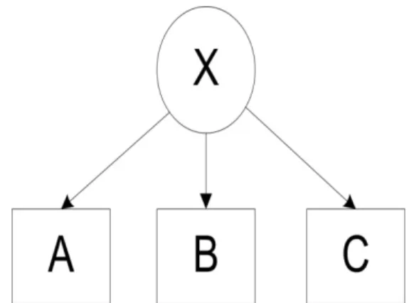
the model estimates to be valid. The key assumption in LCA is local independence. If A, B,
and C are three indicators for the latent variable X, then A, B, and C are called locally
independent if, and only if,
| | | |
| | | |
ABC X A X B X C X abc x a x b x c x
π =π π π (2.1)
where πa xA X|| is the conditional probability that A = a given X = x and πabc xABC X|| ,πb xB X|| , πc xC X|| and
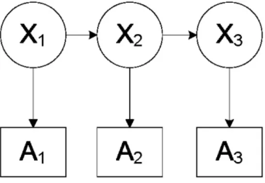
have analogous definitions. Figure 2.1 is a path diagram representing equation 2.1,
illustrating the relationship between the latent variable and its indicators. The right-hand side
of equation (2.1) is known as the measurement component of the latent class model (Bassi,
Hagenaars, Croon, & Vermunt, 2001; Hagenaars, 1998). If this equation fails to hold, the
indicators are locally dependent. Failure of local independence assumptions to hold will
cause poor model fit, create bias in the parameter estimates, and make the standard errors for
the estimates too large (Pepe & Janes, 2007; Sepulveda, Vicente-Villardon, & Galindo,
Figure 2.1 Path diagram for LC model with three indicators and no grouping variables.
This chapter focuses on the root causes of local dependence, their affects on
parameter estimation, diagnostic approaches, and model specifications that correct for one or
more of these causes. To simplify the exposition, my study is confined to sensitive outcomes.
A sensitive outcome is an event for which respondents have a negligible probability of
providing false positive responses. Such events are very important in the study of socially
undesirable phenomenon (e.g., alcohol abuse, sexual misconduct, or drug abuse). For
instance, it is unlikely that people would indicate using marijuana if they do not use it, but it
is more likely that people would indicate not using marijuana when they really do. Such
outcomes are particularly interesting to survey practitioners because respondents do not
always provide truthful answers. Furthermore, although four or five indicators usually
improve the parameter estimates from an LCM, this may be infeasible in some surveys
because of respondent burden, costs, and questionnaire length constraints. For this reason, the
focus in this paper is on three-indicator models because these are most commonly used in
surveys.
2.2.1 Motivation
Although it has been established that local independence is the critical assumption for
root causes of local dependence are and whether these various aspects affect model estimates
differently. Local independence is violated if any of the following three conditions occur:
• Bivocality. Suppose A is an indicator for X, and B is an indicator for Y. If πx yX Y|| <1
for x = y (i.e., X and Y can disagree), then A and B are bivocal (Alwin, 2007).
Bivocal indicators measure two different latent constructs rather than one. For
example, two indicators A and B, where A is past 6-month marijuana use and B is
past month marijuana use, are bivocal because they do not cover the same time
period. A necessary condition for local independence is | | =1
X Y x y
π for x = y referred
to as univocality.
• (Behavioral) correlated error. Suppose indicator A precedes indicator B in the
interview. Their errors will be correlated if respondents who respond erroneously
to indicator A have a greater (or lesser) probability of responding erroneously to
indicator B than respondents who responded accurately. Mathematically, this can
be written as | | 2|21 2|11
B AX B AX
π ≠π , or | |
1|11 1|21
B AX B AX
π ≠π . For instance, people who do not
want interviewers to know about their drug use will falsify any item dealing with
drug use with a greater probability than people who are independently answering
each item. Uncorrelated error is a necessary condition for local independence.
• Latent heterogeneity. Let H denote a grouping variable such that within the
categories of H πa xhA XH|| is homogeneous (i.e., the error probabilities are
homogeneous within each level of H), and suppose thatπa xhA XH|| ≠πa xA X|| . This implies
(2011) shows, this condition, referred to as latent heterogeneity, violates the
assumption of local independence.
Each of these three types of model failures may bias the parameter estimates,
although the magnitudes of the biases may vary in somewhat predictable ways (Sepulveda et
al., 2008). Furthermore, some indicators may be more prone to local dependence than others
and, thus, deciding which indicators to include in a survey can have a major impact on the
resulting LCM estimates.
I illustrate the effects of local dependence using the 2007 National Inmate Survey
(NIS) of prisons; a nationally representative survey of prison inmates that estimated the
12-month prevalence of sexual victimization in prisons (Beck & Harrison, 2007). Sexual
victimization is split into victimization by another inmate (inmate-on-inmate) and
victimization by a staff member (staff-on-inmate). The survey embedded five indicators for
each type of victimization in the questionnaire. Table 2.1 provides the wording of the five
indicators for inmate-on-inmate victimization, which is the primary outcome variable for this
paper. In my analysis, the latent variable represents the respondent’s true inmate-on-inmate
victimization status for the previous 12 months. This is an example of a sensitive outcome
because the false positive probability is expected to be negligibly small (i.e., it is unlikely
that people would claim to be sexually victimized when they were not). On the other hand, I
expect the false negative probability to be substantial because truly victimized inmates might
indicate that they were not victimized because of the traumatic nature of the experience or
fear of reprisal from the perpetrator.
Based on a substantive review of the items in Table 2.1, comparing the language of
indicators A, B, and C are univocal for “sexual assault.” However, indicators D and E have a
different underlying latent variable since they address specific sexual acts (e.g., oral or anal
sex) and do not ask about general types of sexual contact. Thus, the set of indicators A, B, C,
D, and E are bivocal since they jointly measure two distinct latent variables. Since D and E ostensibly measure a different latent variable than A, B, and C, a model specifying a single
latent variable will be misspecified and the parameter estimates will be biased to some
extent.
Table 2.1 Definition of NIS LCA Indicators for Inmate-on-Inmate Sexual Victimization
Indicator Definition
A In the past 12 months or since you’ve been at the facility (if less than 12 months) has another inmate
done the following?
• Use physical force to touch your butt, thighs, or penis in a sexual way? (male only)
• Without physical force, use pressure to touch your butt, thighs, or penis in a sexual way? (male
only)
• Use physical force to touch your butt, thighs, breasts, or vagina in a sexual way? (female only)
• Without physical force, use pressure to touch your butt, thighs, breasts, or vagina in a sexual
way? (female only)
• Use physical force to make you give or receive a handjob? (male only)
• Without physical force, use pressure to make you give or receive a handjob? (male only)
• Use physical force to make you give or receive oral sex?
• Without physical force, use pressure to make you give or receive oral sex?
• Use physical force to make you have vaginal sex? (female only)
• Without physical force, use pressure to make you have vaginal sex? (female only)
• Use physical force to make you have anal sex?
• Without physical force, use pressure to make you have anal sex?
• Use physical force to make you have some other type of sex not asked about?
• Without physical force, use pressure to make you have some other type of sex not asked about?
= 1 if yes = 2 if no
B In the past 12 months or since you’ve been at the facility (if less than 12 months), did another inmate
use physical force, pressure you, or make you feel that you had to have any type of sex or sexual contact in?
= 1 if yes = 2 if no
C How long has it been since another inmate in this facility used physical force, pressured you, or made
you feel that you had to have any type of sex or sexual contact?
= 1 if past 12 months or since arrived at the facility (if less than 12 months) = 2 if more than 12 months or never
Table 2.1 Definition of NIS LCA Indicators for Inmate-on-Inmate Sexual Victimization (cont.)
Indicator Definition
D MALE: In the past 12 months or since you’ve been at the facility (if less than 12 months), did
another inmate use physical force, pressure you, or make you feel that you had to have oral or anal sex?
FEMALE: In the past 12 months or since you’ve been at the facility (if less than 12 months), did another inmate use physical force, pressure you, or make you feel that you had to have oral, vaginal, or anal sex?
= 1 if yes = 2 if no
E MALE: How long has it been since another inmate in this facility used physical force, pressured you,
or made you feel that you had to have oral or anal sex?
FEMALE: How long has it been since another inmate in this facility used physical force, pressured you, or made you feel that you had to have oral, vaginal, or anal sex?
= 1 if past 12 months or since arrived at the facility (if less than 12 months) = 2 if more than 12 months or never
With five indicators, 10 standard three-indicator LC models are possible, which
correspond to all possible combinations of three indicators from the five available. These 10
models, which are listed in Table 2.2, all have the form
| | | | | |
ABC X A X B X C X
abc x a x b x c x
x
π =
∑
π π π π (2.2)for indicators A, B, and C (and can be analogously written for other sets of three indicators).
In this chapter, I will denote a model based on the indicators used in the model (e.g., ABC
indicates the model defined in (2.2). As shown in the Table 2.2, estimates of the false
positive probabilities are quite small for all indicators, while estimates of the false negative
probabilities are substantial and vary considerably across the 10 models for the same
indicator, primarily as a result of local dependence. In what follows, I consider model
Table 2.2 NIS Unadjusted Three-Indicator LCM
Prevalence False Negative Rates False Positive Rates
Model Number
Indicators 1
X π | 2|1 A X π | 2|1 B X π | 2|1 C X π | 2|1 D X π | 2|1 E X π | 1|2 A X π | 1|2 B X π | 1|2 C X π | 1|2 D X π | 1|2 E X π
1 ABC 0.0213 0.1684 0.3433 0.1717 0.0030 0.0011 0.0032
2 ABD 0.0157 0.0936 0.1839 0.3977 0.0065 0.0023 0.0022
3 ABE 0.0182 0.1304 0.2639 0.2729 0.0047 0.0016 0.0030
4 ACD 0.0198 0.0977 0.1794 0.5197 0.0029 0.0046 0.0022
5 ACE 0.0196 0.1878 0.0783 0.2780 0.0049 0.0028 0.0020
6 ADE 0.0162 0.1620 0.3666 0.1525 0.0072 0.0014 0.0025
7 BCD 0.0165 0.1669 0.1585 0.4388 0.0013 0.0070 0.0024
8 BCE 0.0172 0.2921 0.0507 0.2031 0.0029 0.0045 0.0024
9 BDE 0.0148 0.2352 0.3169 0.1405 0.0038 0.0016 0.0035
10 CDE 0.0151 0.1201 0.4142 0.0206 0.0076 0.0028 0.0013
In the following sections, three questions will be explored:
1. How does local dependence bias parameter estimates and which parameter
estimates are most affected?
2. How can model diagnostics be used to detect local dependence?
3. How can local dependence be corrected in the three-indicator LCM?
To answer the first question, expeculation1 (Biemer, 2011) will be used to illustrate
the effects of the various types of local dependence on the parameter estimates. To address
the second and third question, I examine the current literature and propose a process by
which a three-indicator model can be tested for local dependence and what corrective steps
can be taken if dependence is identified.
1Expeculation creates an input data table with frequencies that are equal to the expected cell
frequencies under the assumed population model. This technique is appropriate if interest is only on the expected values or biases of the estimators rather than their standard errors or sampling
I then apply my proposed process on data from the NIS. I look at all 10
three-indicator models and use my approach to assess and correct for local dependence. To assess
the effectiveness of my method, I compare my results to the estimates from the full
five-indicator model, which I treat as a gold standard.
2.3 Simulations
The primary focus in this chapter is on the biasing effects of local dependence, not
variance. Therefore, I will use expeculation (Biemer, 2011) rather than Monte Carlo
simulation. To apply expeculation in the study of local dependence, I first specify a
population model that is the standard LCM except that it includes some violation of local
independence (i.e., bivocality, heterogeneity, or behavioral correlation). The standard LCM is
then fitted to the expected cell frequencies from this population model. The difference
between an estimate from the standard LCM and the corresponding parameter from the
population model is a bias in the estimate induced by the local independence violation.
2.3.1 Bivocality
If A is a dichotomous indicator for the latent variable X and B is a dichotomous
indicator for the latent variable Y, then A and B are univocal if the correlation between X and
Y is 1. Otherwise, A and B are bivocal. If I assume that π π= xX =πYyfor x = y = 1, then the
correlation between X and Y can be derived as
(
)
1|1|,
1
X Y
xy
Corr X Y ρ π π
π
−
= =
− (2.3)
This assumption is reasonable if the two bivocal measures are estimating similar outcomes
since one would expect their prevalence to be similar. If π1|1X Y| =1 then X and Y are identical
variable and A and B are bivocal. Note that π1|1X Y| =ρxy
(
1−π)
+π and π2|2X Y| =ρ πxy + −(
1 π)
and thus the expected frequency, mabc, of the cell (a,b,c) of the ABC table can be written as
| | | | | | | |
A X B X C Y Y X X
abc a x b x c y y x x
x y
m =N
∑∑
π π π π π (2.4)To study the impact of bivocality on the error standard LCM estimates, a
three-indicator model was fit for values of ρxyin the range 0≤ρxy ≤1 at 0.1 increments. The bias
in each parameter was computed as the difference between the parameter estimates from the
standard model and population model. For each case considered, the false negative
probability was moderate to large (varying in the range of 0.1≤π2|1≤0.3), while the false
positive probability was negligible (π1|2=0.01) for each of the three indicators. Three values
of the prevalence probability were considered: π =0.02, π =0.05, and 0.1
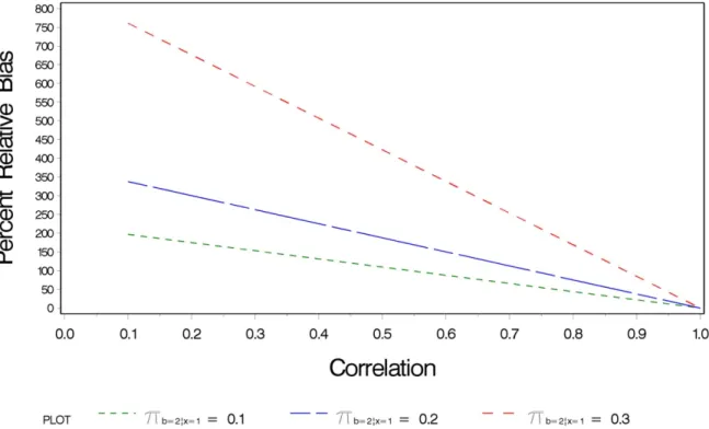
Figure 2.2 displays the percent relative bias in the bivocal indicator by correlation
level for three different false negative rates when π =0.02. Similar results were found when
0.05 =
π and π =0.10. These results suggest that the bivocal indicator (C, which is an
indicator of Y) behaves like a poor indicator of X in the analysis. For example, the estimates
of the false negative probabilities, | 2|1
C X
π , are biased, and, further, the bias is inversely
proportional to the correlation between X and Y. Because I incorporated an additional latent
variable in my model, I fixed the false positive rate to ensure identifiability. Surprisingly,
bivocality in one indicator does not bias error parameters associated with the two univocal
Figure 2.2 Relative bias in the false negative rate of a bivocal indicator by correlation level between the latent variables X and Y.
2.3.2 Correlated Error
If A and B are dichotomous indicators for the latent variable X, then correlated error
can be thought of as the correlation between A and B given X. This correlation can be
expressed as
(
)
1|1| 1|1|(
) (
)
1|2| 1|2|(
)
| | | | |
2|1 2|1 2|2 2|2
, | 1 1 1
A X B X A X B X
ab x A X B X A X B X
Corr A B X ρ x π π λ x π π λ
π π π π
= = − + − − , (2.5)
where
| 1|1 | 1|
B AX x B X
x
π λ
π
= for x = 0,1. Note that when λ=1, ρab x| =0 and classification errors are
uncorrelated errors; otherwise, A and B are conditionally correlated. The expected cell
frequencies can be written as
| | | | | |
X A X B X C X
abc x a x b x c x
x
m =N
∑
π π π π λ (2.6)To demonstrate the effects of behavior correlation on the estimates, a population
model with λ≠1 was used to generate the cell frequencies for the ABC table. Then the
standard LCM was fit to these data. The bias induced by the behavior correlations was
estimated by the difference between the standard LCM estimates and the corresponding
parameters of the population model. As before, for each case considered, the false negative
probability was moderate to large (varying in the range of 0.1≤π2|1≤0.3), while the false
negative probability was negligible (π1|2=0.01) for each of the three indicator. Three values
of the prevalence probability were considered: π =0.02, π =0.05, and 0.1
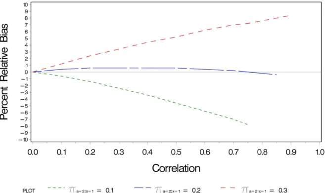
The results of the expeculation found that behavior correlation biases all the
parameter estimates, not just those associated with the two indicators having correlated
errors. Figure 2.3 shows that, for the prevalence probability, the magnitude of the relative
bias usually increases as ρab x| increases; however, the direction of the bias depends on the
magnitude of the false negative probability. Specifically, when the false negative probability
is either small (i.e., 0.1) or large (i.e., 0.3), the magnitude of bias increases with increasing
|
ab x
ρ . However, when the false negative probability is at a moderate level (i.e., 0.2), the bias
varies slightly around 0 regardless of ρab x| . This phenomenon is caused by the canceling
effects of false positive and false negative classifications. When the false negative probability
is small, the number of false positives overwhelms the number of false negatives causing a
negative bias. When the false negative probability is large, the opposite effect occurs.
However, when the false negative probability is at a moderate level, the number of false
negative and false positive classifications are equalized and the bias is close to 0. I obtained
For the classification error rates, the level of bias depends on the magnitude of the
error. For example, for the false negative rate, the relative bias is greatest when the actual
false negative rate is smallest (i.e., 0.1). The relative bias then decreases as the actual false
negative rate increases. However, the false positive rate, which is fixed at a negligible level,
acts in an opposite fashion, having the largest relative bias when the false negative rate is
largest (i.e., 0.3) and smallest when the false negative rate is smallest (i.e., 0.1). Similar
results were obtained for all prevalence levels examined.
Figure 2.3 Relative Bias in Estimated Prevalence Probability due to Correlated Error as a Function of the Correlation and False Negative Probability
2.3.3 Group Heterogeneity
Suppose that the error probabilities vary across the categories of an unobserved,
dichotomous grouping variable H, thus inducing heterogeneity, but are homogeneous within
serve as a proxy for H in the LCM (i.e., G is selected so that πi xhI XH|| ≅πi xgI XG|| when g = h for all
indicators, I =A, B, and C). Consider the LCM with cell probabilities | | | | | | | |
GABC G X G A XG B XG C XG
gabc g x g a xg b xg c xg
x
π =
∑
π π π π π . (2.7)The ability of the grouping variable G to account for the heterogeneity depends upon its
correspondence with the latent variable H. Thus, the biasing effects of heterogeneity on the
model estimates can be expressed as a function of the correlation between G and H. The
greater the correspondence between G and H, the better the ability of G to explain the
unobserved heterogeneity induced by H, and the smaller will be the bias because of
heterogeneity. This correlation can be expressed as
(
)
(
)
(
) (
)
| 1 1|1 1
1 1 1 1
Corr , = =
1 1
G H G H
GH
G G H H
G H ρ π π π
π π π π
−
− − . (2.8)
If I assume that π1G =π1H andπ1|1G H| =1 (i.e., G is essentially identical to H), then ρGH =1 and
the heterogeneity is full accounted for by equation (2.8). However, if either π1G ≠π1H or
| 1|1 1
H G
π < , then G is not a perfect proxy for H, ρGH ≠1, and the model is misspecified. To fix
the ideas, I assumed that π1G =π1H =π* and focused on the case in which 1|1| 1
G H
π < . Then
equation (2.8) can be rewritten as
| * 1|1 * = 1 H G GH π π ρ π − − (2.9)
and thus, | * *
1|1 (1 ) +
H G
GH
π = −π ρ π . Therefore, given π*
and ρGH, the joint distribution of H
Using expeculation, I can demonstrate that the biasing affects group heterogeneity for
any values of π*
and ρGHthrough the expression
| | | | | | | | | |
G G H X H A HX B HX C HX
gabc g g h x h a hx b hx c hx
h x
m =N
∑∑
π π π π π π (2.10)for expected cell frequencies for the GABC table. I then fit the model in equation (2.7) to
evaluate the bias in using G as a proxy for H.
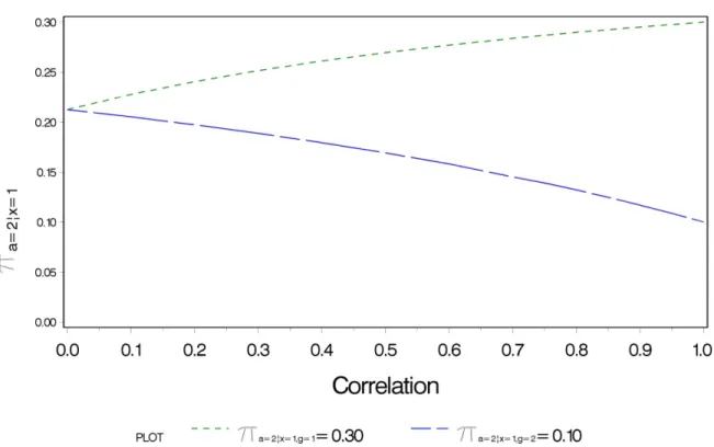
Table 2.3 presents the assumptions used to distinguish the two levels of H, where, for
illustrative purposes, H represents the risk level of a person that can be high or low. For
purposes of the simulation, I assumed one level would contain the respondents in the
high-risk population, and the other level would contain the respondents in the low-high-risk population.
Because of this assumption, the true prevalence rate was set to be higher in the high-risk
group than in the low-risk group. Furthermore, I assumed the false negative rate would be
higher in the high-risk group because those respondents would have a higher sensitivity to
the questions, leading to the high-risk group having a greater chance of falsely indicating that
the event of interest did not occur. Because I assumed a sensitive outcome, the false positive
rate was assumed to be small and the same in each level.
Table 2.3 Assumptions Used in Expeculation of Group Heterogeneity
Assumption
Parameter High-Risk Group Low-Risk Group
True prevalence 0.10 0.02
False negative rate 0.30 0.10
False positive rate 0.01 0.01
The results of the expeculation found that as ρGH increases, both the prevalence and
the false negative rate for each group converged such that when ρGH =0, the two rates were
two groups. The false negative rates converged to something higher than the weighted
average. Figure 2.4 illustrates how the rates converged for the false negative rate.
Figure 2.4 False negative rate in indicator by group as correlation between G and H increases.
2.3.4 What I Learned
My simulation study found that all three types of local dependence bias the model
estimates, but in different ways. A bivocal indicator acts like a poor indicator, which, if too
poor, can lead to an unidentifiable model because there are essentially only two indicators.
Correlated errors affect both the prevalence rates and the classification error rates. The
resulting bias can be large depending on the level of correlation. Group heterogeneity can
lead to a bias in the classification errors. In a three-indicator model, a highly uncorrelated
bivocal indicator may be the most problematic since it affects identifiability. However, a
mildly bivocal indicator only biases the error rates for that indicator. Correlated errors and