The number of primary events per variable affects estimation of the
subdistribution hazard competing risks model
Peter C. Austin
a,b,c,*
, Arthur Allignol
d, Jason P. Fine
e,faInstitute for Clinical Evaluative Sciences, G106, 2075 Bayview Avenue, Toronto, Ontario M4N 3M5, Canada
bInstitute of Health Management, Policy and Evaluation, University of Toronto, 155 College Street, Toronto, Ontario M5T 3M6, Canada cSchulich Heart Research Program, Sunnybrook Research Institute, 2075 Bayview Avenue, Toronto, Ontario M4N 3M5, Canada
dInstitute of Statistics, Ulm University, Helmholtzstr. 20, Ulm 89081, Germany
eDepartment of Biostatistics, University of North Carolina, 135 Dauer Drive, 3101 McGavran-Greenberg Hall, CB #7420 Chapel Hill, NC 27599-7420, USA fDepartment of Statistics & Operations Research, University of North Carolina, 318 Hanes Hall, CB# 3260, Chapel Hill, NC 27599-3260, USA
Accepted 10 November 2016; Published online 12 January 2017
Abstract
Objectives: To examine the effect of the number of events per variable (EPV) on the accuracy of estimated regression coefficients, standard errors, empirical coverage rates of estimated confidence intervals, and empirical estimates of statistical power when using the Fi-neeGray subdistribution hazard regression model to assess the effect of covariates on the incidence of events that occur over time in the
presence of competing risks.
Study Design and Setting: Monte Carlo simulations were used. We considered two different definitions of the number of EPV. One included events of any type that occurred (both primary events and competing events), whereas the other included only the number of pri-mary events that occurred.
Results: The definition of EPV that included only the number of primary events was preferable to the alternative definition, as the num-ber of competing events had minimal impact on estimation. In general, 40e50 EPV were necessary to ensure accurate estimation of
regres-sion coefficients and associated quantities. However, if all of the covariates are continuous or are binary with moderate prevalence, then 10 EPV are sufficient to ensure accurate estimation.
Conclusion: Analysts must base the number of EPV on the number of primary events that occurred. Ó2017 The Author(s). Published by Elsevier Inc. This is an open access article under the CC BY-NC-ND license (http://creativecommons.org/licenses/by-nc-nd/4.0/).
Keywords:Survival analysis; Competing risks; Subdistribution hazard model; Sample size; FineeGray regression model; Events per variable
1. Introduction
Quantifying the occurrence of an adverse event or outcome over time is an important issue in clinical medi-cine and public health research. There is an increasing in-terest in the incidence of nonfatal events (e.g., incidence of heart disease, occurrence of an infection) or the inci-dence of cause-specific mortality (e.g., inciinci-dence of death due to cardiovascular disease or death due to cancer). In such settings, the presence of competing risks must be taken into account when assessing the effect of prognostic factors on the incidence of an outcome over time. A competing risk is an event whose occurrence precludes the occurrence of the event of interest[1e6]. For instance, when evaluating the effect of risk factors on the incidence of death due to cardiovascular disease, death to noncar-diovascular causes serves as a competing risk because subjects who die of a noncardiovascular cause
Funding: This study was supported by the Institute for Clinical Evalu-ative Sciences (ICES), which is funded by an annual grant from the Ontar-io Ministry of Health and Long-Term Care (MOHLTC). The opinOntar-ions, results, and conclusions reported in this paper are those of the authors and are independent from the funding sources. No endorsement by ICES or the Ontario MOHLTC is intended or should be inferred. This research was supported by an operating grant from the Canadian Institutes of Health Research (CIHR) (MOP 86508). Dr. Austin was supported by Career Investigator awards from the Heart and Stroke Foundation. The Enhanced Feedback for Effective Cardiac Treatment (EFFECT) data used in the study were funded by a CIHR Team Grant in Cardiovascular Outcomes Research (CTP 79847 and CRT43823). These data sets were linked using unique, encoded identifiers, and analyzed at the Institute for Clinical Eval-uative Sciences (ICES).
Conflict of interest: None.
* Corresponding author. Tel.: (416)-480-6131; fax: (416)-480-6048. E-mail address:[email protected](P.C. Austin).
http://dx.doi.org/10.1016/j.jclinepi.2016.11.017
0895-4356/Ó2017 The Author(s). Published by Elsevier Inc. This is an open access article under the CC BY-NC-ND license (http://creativecommons.org/
licenses/by-nc-nd/4.0/).
What is new?
Key findings
The number of type 1 events (primary events) was more important than the number of events of any type for assessing the number of events per variable (EPV) when estimating a subdistribution hazard model.
Forty to 50 EPV are necessary to ensure accurate estimation of regression coefficients and associated quantities.
If all of the covariates are continuous or are binary with moderate prevalence, then 10 EPV are suffi-cient to ensure accurate estimation.
What this adds to what was known?
Previous research has examined the number of EPV necessary to fit logistic regression models (bi-nary outcomes) or a Cox proportional hazards models (survival outcomes in the absence of competing risks). The current research extends the findings of these earlier studies to the setting in which competing risks are present.
What is the implication and what should change now?
Authors and analysts need to be aware that the number of type 1 events (or the primary event of interest) is the key number when determining the number of EPV and whether there are an adequate number of events for fitting the desired subdistribu-tion hazard model.
(e.g., cancer) are no longer at risk of death due to cardio-vascular disease.
Na€ıve use of the conventional Cox proportional hazards model that censors the competing event leads to biased estimates of the effect of covariates on incidence in the presence of competing risks [2,3,7]. In response, Fine and Gray[8]developed the subdistribution hazard model which allows one to model the effects of covariates on the cumulative incidence function in the presence of competing risks. It is increasingly being acknowledged that the subdistribution hazard model should be used when evaluating incidence of an outcome over time in the competing risks setting[9].
Peduzzi et al. published an influential series of articles examining the effect of the number of events per variable (EPV) on the accuracy of estimation of regression coeffi-cients for the logistic regression model and for the Cox proportional hazards model in the absence of competing risks[10e12]. For a logistic regression model for use with
binary outcomes, the number of events was defined to be the smaller of the number of events and the number of nonevents (or the smaller of the number of successes and the number of failures). For a Cox proportional haz-ards regression model, the number of events was defined as the number of subjects for whom an event was observed to occur (i.e., the number of noncensored sub-jects). Their studies used simulations based on 673 pa-tients enrolled in a trial comparing medical and surgical management of coronary artery disease. Based on these simulations, they recommended that at least 10 EPV be observed to enable accurate estimation of the regression coefficients. These papers have been very influential, with the article on logistic regression being cited 1,610 times and the article on the Cox regression model being cited 527 times (source: Science Citation Index; Date accessed: June 16, 2016).
When analyzing survival data in which competing risks are present, there are multiple types of events: the primary event of interest (e.g., death due to cardiovascular causes) and the competing events (e.g., death due to noncardiovas-cular causes). The effects of the number of the different types of events on the accuracy of estimation of the coef-ficients of a subdistribution hazard model have not been explored. The results in Peduzzi et al. are not applicable owing in part to competing events and in part to a nonstan-dard weighting technique in the partial likelihood estima-tion procedure which addresses independent censoring
[8]. Given the increasing use of the subdistribution hazard model for estimating the effect of covariates on incidence in the presence of competing events, the objective of the current paper is to examine the effect of the number of EPV on the accuracy of estimation of the coefficients of a subdistribution hazard model. The paper is structured as follows: in Section2, we describe the design of a series of Monte Carlo simulations to examine the impact of the number of EPV on the accuracy of estimation of regression coefficients for a subdistribution hazard model. In Section
3, we report the results of these simulations. In Section4, we summarize our findings, which differ somewhat from those in Peduzzi et al. and discuss them in the context of the existing literature.
2. Monte Carlo simulationsdmethods
In this section, we describe the design of a series of Monte Carlo simulations to examine the effects of the num-ber of EPV on the accuracy of estimation of the coefficients of a subdistribution hazard model. In Section 2.1, we describe data on patients hospitalized with acute myocar-dial infarction (AMI or heart attack). In Section 2.2, we describe analyses that were conducted using these data to determine parameters for the data-generating process in the subsequent Monte Carlo simulations. In Section 2.3, we describe the data-generating process that was used to
simulate survival data from a specified subdistribution haz-ard model. In Section 2.4, we describe the statistical ana-lyses that were conducted in the simulated data. Finally, in Section2.5, we describe the factors that were allowed to vary in the Monte Carlo simulations.
2.1. Data sources
We used data from the Enhanced Feedback for Effective Cardiac Treatment (EFFECT) Study, which collected detailed clinical data on patients hospitalized with AMI between April 1, 1999, and March 31, 2001 (phase 1), and between April 1, 2004, and March 31, 2005 (phase 2), at 103 hospitals in Ontario, Canada [13]. Data on patient demographics, vital signs and physical examination at presentation, medical history, and results of laboratory tests were collected by trained cardiovascular nurse abstractors using retrospective chart review. For the current study, we restricted the study sample to those patients who were discharged alive from hospital. The initial sample consisted of 15,569 subjects. Four hundred five (2.6%) subjects with missing data on continuous base-line covariates necessary to estimate the subdistribution hazard model were excluded from the current case study, leaving 15,164 patients for analysis (10,063 patients in phase 1 and 5,101 patients in phase 2).
Subjects were linked deterministically, using an encoded version of the patient’s health insurance number to the Vital Statistics database maintained by the Ontario Office of the Registrar General. The Vital Statistics database contains information on date of death and cause of death (based on ICD-9 codes) for residents of Ontario. Each subject was followed for 5 years from the date of hospital discharge for the occurrence of death. For those subjects who died within 5 years of discharge, the cause of death was noted in the Vital Statistics database. For the purposes of these analyses, cause of death was categorized as cardiovascular vs. noncardiovascular causes of death. A total of 4,276 (28%) patients died during the 5 years of follow-up. Of these, 2,518 (59%) died of cardiovascular causes, whereas 1,758 (41%) died of noncardiovascular causes.
2.2. Empirical analyses in the EFFECT data
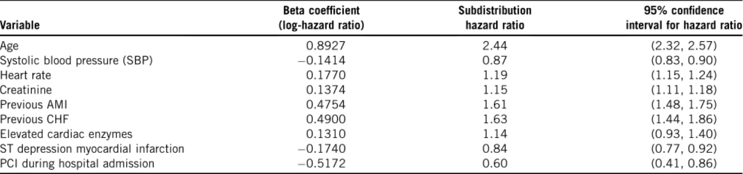
The following nine predictor variables were selected a priori for inclusion in a subdistribution hazard model pre-dicting the occurrence of cardiovascular death: age, heart rate at hospital admission, systolic blood pressure at admission, initial serum creatinine, history of AMI, history of heart failure, ST depression myocardial infarction, elevated cardiac enzymes, and in-hospital percutaneous coronary intervention. These variables were selected because they are components of the GRACE risk score for predicting mortality in patients with acute coronary syndromes [14]. The first four variables are continuous, whereas the last five are dichotomous. We standardized the four continuous variables so that they had mean zero and unit variance. The prevalences of the five binary vari-ables were as follows: history of AMI (23.6%), history of heart failure (4.8%), ST depression myocardial infarction (43.8%), elevated cardiac enzymes (95.2%), and in-hospital percutaneous coronary intervention (4.0%). Thus, the binary covariates had prevalences that ranged from very low to very high. The estimated regression coeffi-cients, subdistribution hazard ratios, and associated 95% confidence intervals are reported in Table 1. We fit a second subdistribution hazard model for the competing event of noncardiovascular death to estimate the effect of the nine covariates on the CIF of noncardiovascular death.
2.3. Data-generating process
We used the analyses conducted in the previous subsec-tion to inform the parameters used in the Monte Carlo simulations. Our data-generating process was a hybrid approach, in which we used previously described CIFs, but the distribution of the covariates and the effect of co-variates on the two CIFs were determined from empirical analyses of EFFECT data. When simulating event types and event times, we used a method of indirect simulation described by Beyersmann et al. [15] (Section 5.3.6), which in turn is based on an approach described by Fine and Gray [8]. In doing so, one only needed to specify
Table 1.Estimated regression coefficients from subdistribution hazard model
Variable
Beta coefficient (log-hazard ratio)
Subdistribution hazard ratio
95% confidence interval for hazard ratio
Age 0.8927 2.44 (2.32, 2.57)
Systolic blood pressure (SBP) 0.1414 0.87 (0.83, 0.90)
Heart rate 0.1770 1.19 (1.15, 1.24)
Creatinine 0.1374 1.15 (1.11, 1.18)
Previous AMI 0.4754 1.61 (1.48, 1.75)
Previous CHF 0.4900 1.63 (1.44, 1.86)
Elevated cardiac enzymes 0.1310 1.14 (0.93, 1.40)
ST depression myocardial infarction 0.1740 0.84 (0.77, 0.92)
PCI during hospital admission 0.5172 0.60 (0.41, 0.86)
Abbreviations:AMI, acute myocardial infarction; CHF, congestive heart failure; PCI, percutaneous coronary intervention.
Age, systolic blood pressure, heart rate, and creatinine were standardized to have mean zero and unit variance. Thus, the associated regression coefficient denotes the change in the log-subdistribution hazard for a one-standard deviation increase in the given continuous variable.
the underlying subdistribution hazard functions and not the cause-specific hazard functions.
We simulated nine baseline covariates for each subject whose distribution would be similar to that of the nine pre-dictors variables described above. Four of the simulated covariates were continuous and were drawn from indepen-dent standard normal distributions (because the four continuous covariates had been standardized to have mean zero and unit variance in the empirical analyses described above). Five of the simulated covariates were binary and were drawn from Bernoulli distributions with parameters equal to the five prevalences described in Section2.2.
For each subject, we simulated a time-to-event outcome from an underlying subdistribution hazard model. The coefficients of the two underlying subdistribu-tion hazard models were equal to those obtained in the empirical analysis described in Section2.2. The cumula-tive incidence functions for the primary and competing events were those described by Beyersmann et al. [15]
and by Fine and Gray [8]. Further details on simulation of the time-to-event outcome are provided in Section A of Appendix in the Supplemental Material section at
www.jclinepi.com that is available online.
2.4. Statistical analyses in simulated data sets
In each of the simulated data sets, we fit a subdistribu-tion hazard model in which the subdistribusubdistribu-tion hazard of the primary event of interest was regressed on the nine simulated baseline covariates. From the fitted regression model, we extracted the following quantities: (1) the esti-mated regression coefficients; (2) the estiesti-mated standard er-rors of the estimated regression coefficients; (3) the estimated 95% confidence intervals for the estimated regression coefficients; and (4) the statistical significance of the estimated regression coefficients.
We estimated the bias in the estimated regression coeffi-cients across 1,000 simulated data sets from the same scenario along with the relative bias, empirical coverage rates of estimated 95% confidence intervals, mean squared error of the estimated regression coefficients, the ratio of the mean estimated standard error to the empirical standard deviation of the estimated regression coefficients, and empir-ical power. These quantities are described in greater detail in Section B ofAppendix in the Supplemental Materialsection atwww.jclinepi.comthat is available online.
2.5. Design of the Monte Carlo simulations
Our Monte Carlo simulations used a full factorial design in which the following two factors were allowed to vary: the number of EPV and the proportion of subjects with co-variates equal to zero who experience the primary event of interest as time gets arbitrarily large (which we denote by p). The expected number of EPV was allowed to take on 10 values: from 5 to 50 in increments of 5. The parameter
p was allowed to take on eight values: from 0.2 to 0.9 in increments of 0.1. We thus examined 80 (108) different scenarios.
In each scenario, we simulated data sets of size N5 2,000 using the data-generating process described in Section 2.3. Our target was to have 1,000 simulated data sets for analysis in each scenario. If, in a given simulated data set, the estimation procedure for fitting the subdistribu-tion hazard model did not converge, then that simulated data set was discarded and a replacement data set was simulated. Thus, for a given scenario, we continued to generate simulated data sets until we obtained 1,000 data sets in which the estimation procedure for the subdistribu-tion hazard model converged.
We repeated the complete set of Monte Carlo simula-tions twice because the total sample size needed for a fixed number of EPV differed depending on how the number of EPV was defined. In the first set of simulations, the number of EPV was based on the number of events of either type that occurred. In the second set of simulations, the number of EPV was based on the number of primary events (events of type 1) that occurred.
All simulations and statistical analyses were conducted using the R statistical software package [16] (version 3.1.2). The subdistribution hazard models were fit using the crr function in the cmprsk package (version 2.2-6).
3. Monte Carlo simulationsdresults
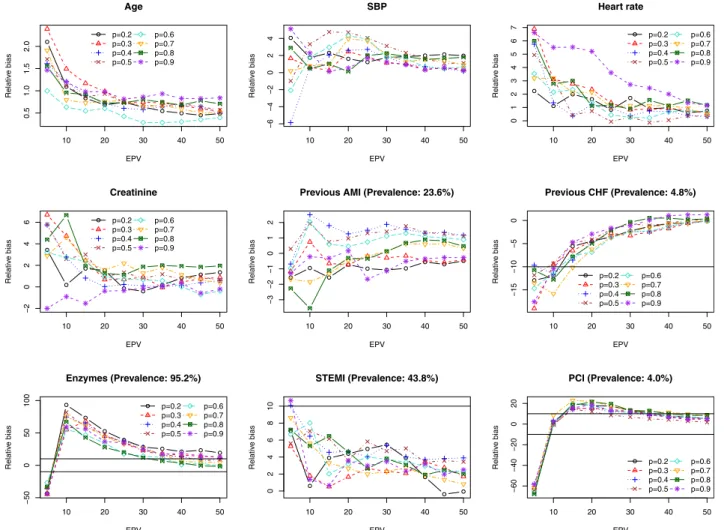
The results of the Monte Carlo simulations are reported graphically inFigures 1 to 4. Each figure consists of nine panels, one for each of the covariates in the subdistribution hazard model. In each panel, we describe the relationship between a given performance measure (e.g., percent bias in the estimated regression coefficient) and the number of EPV for the covariate in question. Each figure contains eight lines, one for each of the different values of the parameter p (the proportion of subjects with covariate values equal to zero for whom a type 1 event was observed to occur ast/N).
The relationship between the number of EPV and the number of data sets that had to be simulated to obtain 1,000 simulated data sets in which the subdistribution hazard model converged is discussed in Section C ofAppendix in the Supplemental Materialsection that is available online.
3.1. Number of EPV based on the number of events of any type that occurred
In this section, we discuss the results of the simulations when the number of EPV was based on the number of events of any type (i.e., type 1 events and type 2 events) that were observed to occur.
As these results are based on the number of events of any type that occurred, it is important to be aware of the
relative frequency of the different types of events that occurred. In each iteration of each scenario, we determined the ratio of the number of type 1 events that occurred to the number of type 2 events that occurred. We also determined the proportion of observed events that were type 1 events. We then determined the mean of this ratio and the mean of this proportion across the 1,000 iterations. The left panel of Fig. S2 in the Supplemental Material at www.jclinepi. com that is available online describes the mean ratio of the number of primary events to competing events across the different scenarios. The right panel of Fig. S2 at
www.jclinepi.comdescribes the mean proportion of events that were type 1 events across the different scenarios. As would be anticipated, the ratio and the proportion of type 1 events increased asp increased.
The relationship between the relative bias and number of EPV is reported inFig. S3 in the Supplemental Materialat
www.jclinepi.comthat is available online. On each panel, we have superimposed horizontal lines denoting relative biases of 10% and 10%, under the subjective assessment that an absolute relative bias of less than 10% is of lesser concern. For the four continuous variables (age, systolic
blood pressure, heart rate, and creatinine), the absolute rela-tive bias was almost always less than 10% even when the number of EPV was as low 5. For two of the three binary covariates whose prevalence was either very low or very high, the magnitude of the relative bias tended to be very large when the number of EPV was low. To improve the interpretability of the plots, we truncated the vertical axis at an absolute relative bias of 100%. For the binary covari-ates, the number of EPV had to be substantially larger to have minimal bias in estimating the regression coefficients. A substantially higher number of EPV was required when the prevalence of the covariate was either very low or very high, compared to when the prevalence was closer to 0.5. For a given number of EPV, the absolute relative bias tended to decrease as p increased (i.e., as the probability of experiencing a type 1 event for a subject with covariates equal to zero increased). Whenpwas low and the covariate had a very high prevalence, moderate bias was observed even when the number of EPV was equal to 50.
The relationship between the number of EPV and the ratio of the mean estimated standard error to the standard deviation of the estimated regression coefficients is 10 20 30 40 50
0.5
1.0
1.5
2.0
EPV
Relativ
e bias
Age
p=0.2 p=0.3 p=0.4 p=0.5
p=0.6 p=0.7 p=0.8 p=0.9
10 20 30 40 50
−6
−4
−2
0
2
4
EPV
Relativ
e bias
SBP
10 20 30 40 50
01234567
EPV
Relativ
e bias
Heart rate
p=0.2 p=0.3 p=0.4 p=0.5
p=0.6 p=0.7 p=0.8 p=0.9
10 20 30 40 50
−
2
0246
EPV
Relativ
e bias
Creatinine
p=0.2 p=0.3 p=0.4 p=0.5
p=0.6 p=0.7 p=0.8 p=0.9
10 20 30 40 50
−3
−2
−1
0
1
2
EPV
Relativ
e bias
Previous AMI (Prevalence: 23.6%)
10 20 30 40 50
−15
−
10
−5
0
EPV
Relativ
e bias
Previous CHF (Prevalence: 4.8%)
p=0.2 p=0.3 p=0.4 p=0.5
p=0.6 p=0.7 p=0.8 p=0.9
10 20 30 40 50
−50
0
50
100
EPV
Relativ
e
bias
Enzymes (Prevalence: 95.2%)
p=0.2 p=0.3 p=0.4 p=0.5
p=0.6 p=0.7 p=0.8 p=0.9
10 20 30 40 50
02468
1
0
EPV
Relativ
e
bias
STEMI (Prevalence: 43.8%)
10 20 30 40 50
−60
−
40
−20
0
20
EPV
Relativ
e
bias
PCI (Prevalence: 4.0%)
p=0.2 p=0.3 p=0.4 p=0.5
p=0.6 p=0.7 p=0.8 p=0.9
Fig. 1. Effect of the number of EPV on relative bias. EPV, events per variable; AMI, acute myocardial infarction; PCI, percutaneous coronary inter-vention; SBP, systolic blood pressure.
described inFig. S4 in the Supplemental Materialatwww. jclinepi.comavailable online. For the four continuous vari-ables, this ratio was approximately equal to one when the number of EPV was at least 10. A similar phenomenon was observed for those binary covariates whose prevalence was moderate. However, for those binary covariates with a very low or very high prevalence, a substantially higher number of EPV was necessary for the ratio to be close to one.
The relationship between the number of EPV and empir-ical coverage rates of the estimated 95% confidence inter-vals is described inFig. S5 in the Supplemental Materialat
www.jclinepi.comavailable online. Due to our use of 1,000 iterations per scenario, any empirical coverage rate that was less than 0.9365 or greater than 0.9635 would be statistically significantly different than the advertised rate of 0.95 using a standard normal-theory test and a signifi-cance level of 0.05. Accordingly, we have superimposed horizontal lines denoting coverage rates of 0.9365 and 0.9635 on each panel. In general, once the number of EPV exceeded 15e20, the empirical coverage rates tended to be approximately equal to the nominal rates.
The relationship between the number of EPV and the empirical estimate of statistical power to detect a nonnull hazard ratio is described in Fig. S6 in the Supplemental Material at www.jclinepi.com. As would be expected, in general, statistical power increased with increasing number of EPV. Furthermore, power increased with increasing p. Some aberrant results were observed in the case of binary co-variates for which the prevalence was very low or very high. In these settings, statistical power displayed a U-shaped rela-tionship with the number of EPV. These anomalous findings are likely due to the large biases in estimation that were observed to occur with a low number of EPV.
3.2. Number of EPV based on the number of primary events that occurred
In this section, we discuss the results of the simulations when the number of EPV was based only on the number of primary events that were observed to occur.
The relationship between the relative bias and number of EPV is reported in Fig. 1. For the continuous covariates, very low bias was observed across all values of the number 10 20 30 40 50
0.96
1.00
1.04
EPV
SE/SD r
a
tio
Age
10 20 30 40 50
0.92
0.96
1.00
EPV
SE/SD r
a
tio
SBP
10 20 30 40 50
0.96
1.00
1.04
EPV
SE/SD r
a
tio
Heart rate
10 20 30 40 50
0.94
0.98
1.02
EPV
SE/SD r
atio
Creatinine
10 20 30 40 50
0.94
0
.96
0.98
1.00
EPV
SE/SD r
atio
Previous AMI (Prevalence: 23.6%)
10 20 30 40 50
0.90
0
.95
1.00
1
.05
EPV
SE/SD r
atio
Previous CHF (Prevalence: 4.8%)
p=0.2 p=0.3 p=0.4 p=0.5
p=0.6 p=0.7 p=0.8 p=0.9
10 20 30 40 50
1.0
1
.1
1.2
1
.3
EPV
SE/SD r
atio
Enzymes (Prevalence: 95.2%)
p=0.2 p=0.3 p=0.4 p=0.5
p=0.6 p=0.7 p=0.8 p=0.9
10 20 30 40 50
0.96
0.98
1.00
1.02
EPV
SE/SD r
atio
STEMI (Prevalence: 43.8%)
10 20 30 40 50
0.9
1
.1
1.3
1.5
EPV
SE/SD r
atio
PCI (Prevalence: 4.0%)
p=0.2 p=0.3 p=0.4 p=0.5
p=0.6 p=0.7 p=0.8 p=0.9
Fig. 2. Ratio of mean standard error to empirical SD of sampling distribution. EPV, events per variable; AMI, acute myocardial infarction; PCI, percutaneous coronary intervention; SBP, systolic blood pressure; SD, standard deviation.
of EPV. For binary covariates with moderate prevalence, minimal bias in estimation of the regression coefficients was observed once the number of EPV was at least 10. In general, for binary covariates with a very low or very high prevalence, the number of EPV had to exceed 40e50 before bias was minimal. In a small number of scenarios, the absolute relative bias exceeded 10% even when the number of EPV was equal to 50.
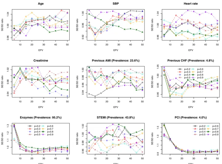
The relationship between the number of EPV and the ratio of the mean estimated standard error to the standard deviation of the estimated regression coefficients is described in Fig. 2. Once the number of EPV was equal to at least 15, then the ratio of these two quantities tended to lie between 0.9 and 1.1, indicating that the model-based estimate of standard error was off by at most 10%.
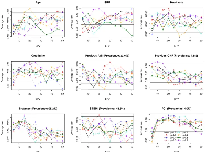
The relationship between the number of EPV and empir-ical coverage rates of the estimated 95% confidence inter-vals is described in Fig. 3. The empirical coverage rates tended to be approximately equal to the nominal rate once the number of EPV was equal to at least 15.
The relationship between the number of EPV and the empirical estimate of statistical power to detect a nonnull
hazard ratio is described inFig. 4. As would be expected, in general, statistical power increased with increasing number of EPV. The value of p had a minimal effect on empirical power. As above, some aberrant results were observed in the case of binary covariates for which the prevalence was very low or very high. In these settings, statistical power displayed a U-shaped relationship with the number of EPV. As above, we hypothesize that these anomalous findings are likely due to the biases in estima-tion that were observed to occur with a low number of EPV.
3.3. Sensitivity analysisdcorrelated covariates
In the primary set of simulations, the nine baseline co-variates were simulated to be independent of one another. We examined the robustness of our findings to this assumption. We repeated the set of simulations in which the number of EPV was based on the number of primary or type 1 events that were observed. When generating the nine baseline covariates, we did so in a manner to induce a pairwise correlation in covariates that reflected what 10 20 30 40 50
0.935
0.945
0.955
0.965
EPV
Co
v
e
rage r
ate
Age
10 20 30 40 50
0.92
0.93
0.94
0.95
0.96
EPV
Co
v
e
rage r
ate
SBP
10 20 30 40 50
0.935
0.945
0.955
EPV
Co
v
e
rage r
ate
Heart rate
10 20 30 40 50
0.93
0
.94
0.95
0.96
EPV
Co
v
e
rage r
a
te
Creatinine
10 20 30 40 50
0.930
0
.940
0.950
0.960
EPV
Co
v
e
rage r
a
te
Previous AMI (Prevalence: 23.6%)
10 20 30 40 50
0.93
0.94
0.95
0.96
EPV
Co
v
e
rage r
a
te
Previous CHF (Prevalence: 4.8%)
10 20 30 40 50
0.940
0.950
0.960
EPV
Co
v
e
rage r
a
te
Enzymes (Prevalence: 95.2%)
10 20 30 40 50
0.940
0
.950
0.960
EPV
Co
v
e
rage r
a
te
STEMI (Prevalence: 43.8%)
10 20 30 40 50
0.92
0.94
0
.96
EPV
Co
v
e
rage r
a
te
PCI (Prevalence: 4.0%)
p=0.2 p=0.3 p=0.4 p=0.5
p=0.6 p=0.7 p=0.8 p=0.9
Fig. 3.Empirical coverage rates of 95% confidence intervals. EPV, events per variable; AMI, acute myocardial infarction; PCI, percutaneous cor-onary intervention; SBP, systolic blood pressure.
was observed in the EFFECT data. The relationship be-tween the number of EPV and relative bias is described in Fig. S7 of the Supplemental Material at www. jclinepi.com available online. Results comparable to those reported above were observed. Comparable results for the other metrics were also observed (results not shown).
3.4. Sensitivity analysisdeffect of estimating the censoring distribution
The estimation procedure for fitting the subdistribution hazard model uses inverse probability of censoring weight-ing. We conducted a sensitivity analysis to determine the impact of estimating the censoring weights on model per-formance. To do so, we used data from the simulations described in Section 3 (in which the number of EPV was based on only the number of primary or type 1 events that occurred). In each simulated data set, we conducted a ‘‘censoring complete’’ analysis, because for each subject, both the event time and the censoring time were known
[17]. To do so, subjects for whom a type 2 event was
observed to have occurred had their event time replaced by their simulated censoring time and their event indicator was changed to indicate that they had been censored at this time. Thus, the only subjects for whom an event was observed to occur were those who experienced a type 1 event (and for whom the simulated type 1 event time was before the simulated censoring time). All other subjects were censored at their randomly generated censoring time. Then, a conventional Cox proportional hazard model was used to estimate the effect of covariates on the incidence of the outcome.
The convergence issues that affected the subdistribution estimation procedure in the presence of a low number of EPV (Fig. S1 at www.jclinepi.com) were not present for the censoring complete analysis. The conventional Cox model converged in each of the first 1,000 simulated data sets in each of the 80 scenarios. When conducting a censoring complete analysis, the effect of the number of EPV on performance did not differ meaningfully from that of the subdistribution hazard model in those data sets in which convergence was achieved (Section 3.2) (results not shown).
10 20 30 40 50
0.9990 0.9994 0.9998 EPV Po w e r Age p=0.2 p=0.3 p=0.4 p=0.5 p=0.6 p=0.7 p=0.8 p=0.9
10 20 30 40 50
0.2 0.4 0.6 0.8 EPV Po w e r SBP p=0.2 p=0.3 p=0.4 p=0.5 p=0.6 p=0.7 p=0.8 p=0.9
10 20 30 40 50
0.2 0.4 0.6 0.8 1.0 EPV Po w e r Heart rate p=0.2 p=0.3 p=0.4 p=0.5 p=0.6 p=0.7 p=0.8 p=0.9
10 20 30 40 50
0.2 0 .4 0.6 0.8 EPV Po w e r Creatinine p=0.2 p=0.3 p=0.4 p=0.5 p=0.6 p=0.7 p=0.8 p=0.9
10 20 30 40 50
0.3 0 .5 0.7 0.9 EPV Po w e r
Previous AMI (Prevalence: 23.6%)
p=0.2 p=0.3 p=0.4 p=0.5 p=0.6 p=0.7 p=0.8 p=0.9
10 20 30 40 50
0.2 0 .4 0.6 EPV Po w e r
Previous CHF (Prevalence: 4.8%)
p=0.2 p=0.3 p=0.4 p=0.5 p=0.6 p=0.7 p=0.8 p=0.9
10 20 30 40 50
0.02 0.04 0.06 0.08 EPV Po w e r
Enzymes (Prevalence: 95.2%)
10 20 30 40 50
0.1 0 .2 0.3 0.4 EPV Po w e r
STEMI (Prevalence: 43.8%)
p=0.2 p=0.3 p=0.4 p=0.5 p=0.6 p=0.7 p=0.8 p=0.9
10 20 30 40 50
0.0 0 .1 0.2 0 .3 0.4 EPV Po w e r
PCI (Prevalence: 4.0%)
p=0.2 p=0.3 p=0.4 p=0.5 p=0.6 p=0.7 p=0.8 p=0.9
Fig. 4. Empirical power. EPV, events per variable; AMI, acute myocardial infarction; PCI, percutaneous coronary intervention; SBP, systolic blood pressure.
4. Discussion
Estimating the incidence of an adverse event or outcome that occurs over time is an important issue in clinical med-icine and population health research. Accurate estimation of the effect of covariates on incidence requires that competing risks be adequately accounted for. The FineeGray subdistribution hazards model was developed to model the effect of covariates on the CIF, allowing for estimation of the effect of covariates on the incidence of events over time. In the current study, we examined the effect of the number of EPV on the accuracy with which the coefficients of the underlying subdistribution hazard model and their standard errors are estimated. We summa-rize our findings in the following paragraphs and then place these findings in the context of the existing literature.
We explored two different definitions of the number of EPV. The first was based on the number of events of any type that were observed to occur, whereas the second was based on the number of type 1 events that were observed to occur. We would suggest that the latter definition is to be preferred over the former definition. In comparing
Figs. S3 through S6 at www.jclinepi.com with Figs. 1 through 4, one notes that with the former definition, the ef-fect of the number of EPV on estimation depends on the proportion of observed events that were type 1 events. However, with the latter definition, the proportion of observed events that were type 1 events did not have a meaningful impact on the quality of estimation. This sug-gests that the number of type 2 events that occurred did not have a meaningful impact on the estimation of the sub-distribution hazard model. For the remainder of the discus-sion of our results, we will focus on the latter definition of the number of EPV.
We found that estimation of regression coefficients associated with continuous covariates (and associated quantities such as standard errors and confidence intervals) was accurate even when the number of EPV was at small as five. For binary covariates, our findings were more com-plex. The effect of the number of EPV on estimation of regression coefficients (and associated quantities) for binary covariates with a moderate prevalence was similar to its effect on estimation of continuous covariates. How-ever, for binary covariates with a very low prevalence or a very high prevalence, a much higher number of EPV was required for accurate estimation of the regression co-efficients and associated quantities. In some settings, as many as 40e50 EPV was required for estimation of regres-sion coefficients with minimal bias. However, accurate estimation of standard errors was observed once the num-ber of EPV was at least 15. A similar lower bound on the number of EPV tended to result in accurate estimation of confidence intervals. These findings are qualitatively similar to what is known about estimation of continuous and binary covariate effects in other regression models, including the standard proportional hazards model.
We would draw the reader’s attention to the high propor-tion of simulated data sets in which the subdistribupropor-tion hazard model did not converge when the number of EPV was low. When the number of EPV was based only on the number of type 1 events, then the number of EPV had to be at least 15 before the percentage of simulated data sets in which convergence was not achieved was less than 10%. When the number of EPV was equal to 5, then lack of convergence was observed in over 45% of the simulated data sets. This has implications for analysts fitting subdistri-bution hazard models in data sets in which the number of EPV is very low. Not only is there the risk of inaccurate estimates of covariate effects on incidence and incorrect inferences, there is also a substantial risk that the model estimation procedure will fail to converge. In contrast, in a censoring complete analysis using the conventional Cox regression model, lack of convergence was not present. This suggests that in small samples, there may be instability associated with the estimated weight, leading to nonconver-gence in the crr function. Some of the differences in convergence may also be due to the different convergence criteria and the way that convergence is defined in the different software procedures.
Our findings differ somewhat from those of Peduzzi et al. [10]in the context of conventional survival analysis using the Cox proportional hazards model. While admitting that a single threshold for the required number of EPV was difficult to choose, they recommended that a threshold of 10 EPV be used. When considering the subdistribution haz-ard model, we found that a much higher threshold for the number of EPV was necessary to permit accurate estima-tion of regression coefficients. While the presence of competing events and the method of estimation for the sub-distribution hazard model may partially explain differences between our findings and those in Peduzzi et al., differences in the simulation designs may also play a role. However, our observation that the quality of estimation was similar for the conventional subdistribution hazard model and the censoring complete analysis suggests that the weighting in the Fine and Gray model is not responsible for the differ-ences between our findings on the necessary number of EPV and those of Peduzzi et al. This suggests that the dif-ferences in the required number of EPV in our study and those proposed by Peduzzi et al. are mostly due to the simu-lation design and not the additional requirement to model the censoring distribution in the FineeGray model. In terms of design, the two studies are similar in that both sets of simulations were based on an analysis of empirical data of patients with heart disease. The simulations differed in that their data consisted of one continuous variable (number of diseased vessels) and six binary covariates. Apart from one binary covariate with a prevalence of 0.07 (history of CHF), the other five binary covariates in the earlier study had less extreme prevalences[11]. As we observed above, a much larger number of EPV was required when binary covariates had very low or very high prevalence. It is likely
the fact that we considered three covariates with extreme prevalences that resulted in our higher threshold for the required number of EPV. The discrepancy between our findings and those of Peduzzi et al. reflects the observation of Courvoisier et al., who suggested that the required num-ber of EPV depended on the structure of the data and the underlying model [18]. The current scenario reflects what is often observed in clinical settings, in which there are important risk factors whose prevalence is very low, but which need to be incorporated into risk prediction models. Furthermore, our scenario included a mixture of continuous and binary covariates, and the prevalences of the binary co-variates covered the full spectrum of what is typically observed in practice.
In the presence of competing risks, investigators can analyze the effect of covariates on the cause-specific hazard function and on the CIF. Latouche et al. argued that for complete understanding of the event dynamics, one should estimate the effects of covariates on both the cause-specific hazard and the cumulative incidence function [19]. The conventional Cox model examined by Peduzzi et al. can be used for examining the effect of covariates on the cause-specific hazard function, by treating subjects who experience competing events as being censored at the time that the competing event occurred. Based on the earlier work by Peduzzi et al., one would require that a minimum of 10 events of interest occur for each covariate included in the cause-specific hazard model. Based on the findings from the current study, we would recommend that a mini-mum of 40e50 events of the given type be observed per variable when modeling the effect of covariates on the CIF. If one were to follow the recommendation of Latouche et al. and fit both cause-specific and CIF regression models, this suggests that the larger of the two minimum number of EPV would be requireddthat in this setting, one would want a minimum of 40e50 events of the given type per variable.
In conclusion, we recommend that, in general, for accu-rate estimation of regression coefficients (and associated quantities) of a subdistribution hazard model, that 40e50 EPV be observed. However, in some settings, this require-ment can be relaxed substantially. If all of the covariates are continuous or are binary with a moderate prevalence, then the number of EPV can be as low as 10.
Supplementary data
Supplementary data related to this article can be found at
http://dx.doi.org/10.1016/j.jclinepi.2016.11.017.
References
[1] Koller MT, Raatz H, Steyerberg EW, Wolbers M. Competing risks and the clinical community: irrelevance or ignorance? Stat Med 2012;31:1089e97.
[2] Lau B, Cole SR, Gange SJ. Competing risk regression models for epidemiologic data. Am J Epidemiol 2009;170:244e56.
[3] Putter H, Fiocco M, Geskus RB. Tutorial in biostatistics: competing risks and multi-state models. Stat Med 2007;26:2389e430.
[4] Satagopan JM, Ben-Porat L, Berwick M, Robson M, Kutler D, Auerbach AD. A note on competing risks in survival data analysis. Br J Cancer 2004;91:1229e35.
[5] Wolbers M, Koller MT, Stel VS, Schaer B, Jager KJ, Leffondre K, et al. Competing risks analyses: objectives and approaches. Eur Heart J 2014;35:2936e41.
[6] Austin PC, Lee DS, Fine JP. Introduction to the analysis of survival data in the presence of competing risks. Circulation 2016;133:601e9. [7] Wolbers M, Koller MT, Witteman JC, Steyerberg EW. Prognostic models with competing risks: methods and application to coronary risk prediction. Epidemiology 2009;20:555e61.
[8] Fine JP, Gray RJ. A proportional hazards model for the subdistribu-tion of a competing risk. J Am Stat Assoc 1999;94:496e509. [9] Austin PC, Lee DS, D’Agostino RB, Fine JP. Developing
points-based risk-scoring systems in the presence of competing risks. Stat Med 2016;35:4056e72.
[10] Peduzzi P, Concato J, Feinstein AR, Holford TR. Importance of events per independent variable in proportional hazards regression analysis. II. Accuracy and precision of regression estimates. J Clin Epidemiol 1995;48:1503e10.
[11] Peduzzi P, Concato J, Kemper E, Holford TR, Feinstein AR. A simu-lation study of the number of events per variable in logistic regression analysis. J Clin Epidemiol 1996;49:1373e9.
[12] Concato J, Peduzzi P, Holford TR, Feinstein AR. Importance of events per independent variable in proportional hazards analysis. I. Background, goals, and general strategy. J Clin Epidemiol 1995;48: 1495e501.
[13] Tu JV, Donovan LR, Lee DS, Wang JT, Austin PC, Alter DA, et al. Effectiveness of public report cards for improving the quality of cardiac care: the EFFECT study: a randomized trial. J Am Med Assoc 2009;302:2330e7.
[14] Eagle KA, Lim MJ, Dabbous OH, Pieper KS, Goldberg RJ, Van de WF, et al. A validated prediction model for all forms of acute coronary syndrome: estimating the risk of 6-month postdischarge death in an international registry. J Am Med Assoc 2004;291: 2727e33.
[15] Beyersmann J, Allignol A, Schumacher M. Competing Risks and Multistate Models with R. New York: Springer; 2012.
[16] R Core Development Team. R: a language and environment for statistical computing. Vienna: R Foundation for Statistical Computing; 2005: Ref Type: Computer Program.
[17] Zhou B, Latouche A, Rocha V, Fine J. Competing risks regression for stratified data. Biometrics 2011;67:661e70.
[18] Courvoisier DS, Combescure C, Agoritsas T, Gayet-Ageron A, Perneger TV. Performance of logistic regression modeling: beyond the number of events per variable, the role of data structure. J Clin Epidemiol 2011;64:993e1000.
[19] Latouche A, Allignol A, Beyersmann J, Labopin M, Fine JP. A competing risks analysis should report results on all cause-specific hazards and cumulative incidence functions. J Clin Epidemiol 2013;66:648e53.